ORIGINAL ARTICLE: Stephen L. Adler and Brent Doherty, Dynamical Gravastar “Simulated Horizon’’ from TOV Equation Initial Value Problem with Relativistic Matter, arXiv:2309.13380. DOI: https://doi.org/10.48550/arXiv.2309.13380
Article Abstract: We continue the study of “dynamical gravastars’’, constructed by solving the Tolman-Oppenheimer-Volkoff (TOV) equation with relativistic matter, undergoing a phase transition at high pressure to a state with negative energy density, as allowed in quantum theory. Since generation of a horizon-like structure or “simulated horizon’’ occurs at a radius above where the phase transition occurs, it is solely a property of the TOV equation with relativistic matter, for appropriate small radius initial conditions. We survey the formation of a simulated horizon from this point of view. From the numerical solutions, we show that the metric exponent appearing in the TOV equation undergoes an arc tangent-like jump, leading to formation of the simulated horizon. Rescaling the problem to fixed initial radius, we plot the “phase diagram’’ in the initial pressure--initial mass plane, showing the range of parameters where a simulated horizon dynamically forms.
Backstory for this project: Stephen L. Adler, Dynamical Gravastars, Phys. Rev. D 106, 104061 (2022), https://doi.org/10.1103/PhysRevD.106.104061. arXiv:2209.02537.
DISCUSSION: https://community.wolfram.com/groups/-/m/t/2820793
GITHUB: https://gitlab.com/stephenadler/Gravastar
See also: Stephen L. Adler, arXIv:2301.11821 for a simplified version used here.
DISCUSSION: https://community.wolfram.com/groups/-/m/t/2820793
GITHUB: https://gitlab.com/stephenadler/Gravastar
See also: Stephen L. Adler, arXIv:2301.11821 for a simplified version used here.
Observations by the Event Horizon Telescope (EHT) of Sg A* and M87 confirm that each has the expected exterior spacetime geometry of a black hole of mass , with a light sphere at a radius 3M lying outside the Schwarzschild radius of 2M. A key question that remains is whether what lies inside the light sphere is a true mathematical black hole, or a novel type of relativistic star or “exotic compact object”. Two recent papers by Adler (listed above as ‘’backstory’’ ) have presented a theory of “dynamical gravastars’’, based on using as input only the Tolman-Oppenheimer-Volkoff (TOV) equations governing relativistic stars, and an assumed equation of state, with continuous pressure and a jump in the energy density at a pressure pjump, from an external relativistic matter state with energy density equal to three times the pressure, to an interior state with pressure plus energy density summing to a small positive constant. A third article by Adler and Doherty, for which this notebook was written, explores the “dynamical gravastar’’ phenomenon from the point of view of an initial value problem for the exterior region, above the energy density jump, where everything is continuous. It shows that given a sufficiently negative integrated energy density as an initial boundary condition, the TOV equations for relativistic matter generate a horizon-like structure that we call the “simulated horizon”. Thus appearance of the simulated horizon does not depend on fine details of what is happening in the interior region, but only on the sign and magnitude of the integrated energy density at the outer boundary of the interior region, which is what supplies the initial value boundary condition for the exterior region.
M
This notebook was used in Fig. 8 and Tables 1-3 of the Adler-Doherty paper arXiv:2309.13380
In[]:=
pinit=1;eminit=17.99;rmin=50;rmax=140.;kappa=8*Pi;kappa2=4*Pi;
The equation of state is implemented by the function
In[]:=
rho[x_]:=3*x
In using these functions in the differential equation solver, x will always be the pressure .
p[r]
In[]:=
system={p[rmin]pinit,em[rmin]eminit,Derivative[1][em][r]kappa2*r^2*rho[p[r]],Derivative[1][p][r]-(1/2)*(p[r]+rho[p[r]])*(2/r^2)*(em[r]+kappa2*r^3*p[r])/(1-2*em[r]/r)};
Next comes the command NDSolve for the system of equations. First@ extracts scalar values for the interpolating functions, as needed for Nminimize, etc. below.
In[]:=
s=First@NDSolve[system,{p,em},{r,rmin,rmax},PrecisionGoal13,AccuracyGoal13,MaxSteps10^10];
Next is extraction of the solution from the interpolating functions constructed by NDSolve,and computation of certain auxiliary quantities.
In[]:=
pout[r_]:=Evaluate[p[r]/.s];emout[r_]:=Evaluate[em[r]/.s];denomout[r_]:=(1-2*emout[r]/r);nuprimeout[r_]:=(2/r^2)*(emout[r]+kappa2*r^3*pout[r])/denomout[r];
Finally, comes printing and plotting of output from the solution
In[]:=
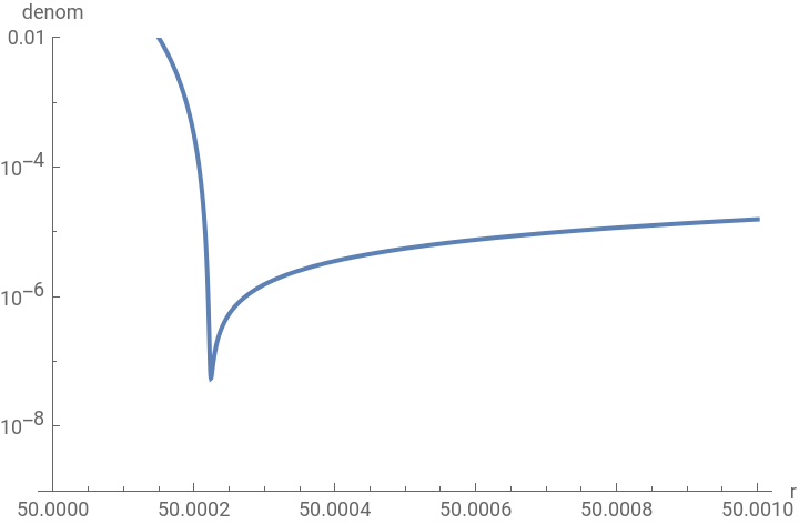
targ=LogPlot[denomout[r],{r,50,50.001},PlotRange{10^-9,.01},AxesLabel->{"r","denom"}]
Out[]=
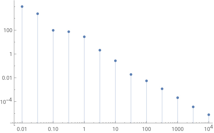
The second number of each pair is 25-minitMAX, where adding 1 to the last significant digit in minitMAX leads to a ‘’stiff’’ diagnostic. This data is then used in the plots below for Fig. 8. of arXiv:2309. 13380:
In[]:=
dataphase1={{.01,(25-24.9998999)^-1},{.03162,(25-24.9996004)^-1},{.1,(25-24.9899999)^-1},{.3162,(25-24.9869469)^-1},{1,(25-24.9651)^-1},{3.162,(25-24.5310)^-1},{10,(25-21.366)^-1},{31.62,(25+26.75)^-1},{100,(25+153)^-1},{316.2,(25+806)^-1},{1000,(25+4640)^-1},{3162,(25+27600)^-1},{10000,(25+126000)^-1}};ListLogLogPlot[dataphase1,Filling->Axis]ListLogLogPlot[dataphase1,Joined->True,FillingAxis,FillingStyleThick,AxesLabel->{"p0","1/(25-m0)"}]
Out[]=
Out[]=
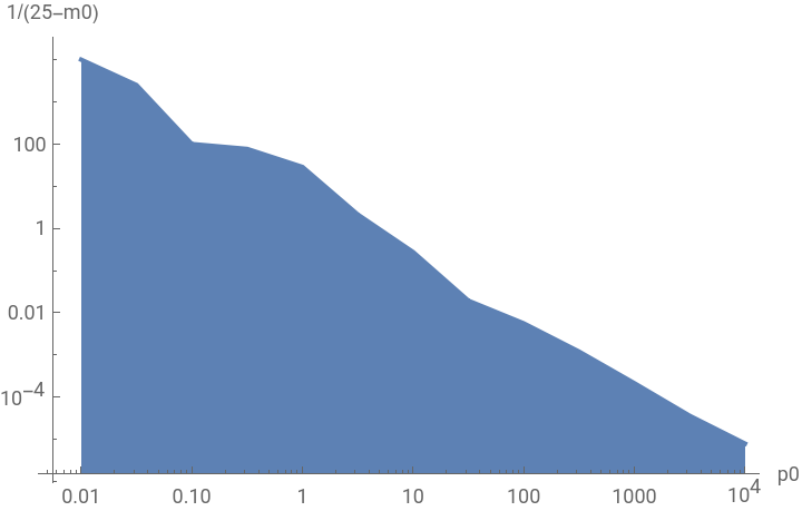
Above figure is Fig . 8
The following computes the minimum and its location in r of the graph labeled "targ" above, as needed for the first line of Table 2 of arXiv:2309. 13380:
In[]:=
NMinimize[{denomout[r],{50.0002≤r≤50.0003}},r]
Out[]=
{5.48175×,{r50.0002}}
-8
10
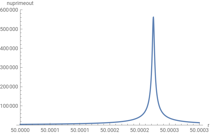
The following is used to compute the full width at half maximum of the graph labeled "newtarg" below, as needed for the first line of Table 2 of arXiv:2309.13380:
In[]:=
NMaximize[{nuprimeout[r],{50.0002≤r≤50.0003}},r,PrecisionGoal6,AccuracyGoal6]
Out[]=
{561716.,{r50.0002}}
The next line divides by 2 to get the half maximum:
In[]:=
561716.503121204`/2
Out[]=
280858.
The next command finds the lower r where nuprimeout equals half the maximum:
lower=FindRoot[nuprimeout[r]-280858.251560602`0,{r,50.0002,50.000223122554054`},MaxIterations10000]

Out[]=
{r50.0002}
The next command finds the upper r where nuprimeout equals half the maximum:
In[]:=
upper=FindRoot[nuprimeout[r]-280858.251560602`0,{r,50.000223122554054`,50.0003},MaxIterations10000]
Out[]=
{r50.0002}
The next line subtracts to find the full width at half maximum:
In[]:=
50.00022620608258`-50.00022003909065`
Out[]=
6.16699×
-6
10
In[]:=
newtarg=Plot[nuprimeout[r],{r,50.000,50.0003},PlotRange{0,6*10^5},AxesLabel->{"r","nuprimeout"}]
Out[]=
CITE THIS NOTEBOOK
CITE THIS NOTEBOOK
Dynamical Gravastar "Simulated Horizon'' from TOV Equation Initial Value Problem with Relativistic Matter
by Stephen L. Adler and Brent Doherty
Wolfram Community, STAFF PICKS, September 27, 2023
https://community.wolfram.com/groups/-/m/t/3022687
by Stephen L. Adler and Brent Doherty
Wolfram Community, STAFF PICKS, September 27, 2023
https://community.wolfram.com/groups/-/m/t/3022687