Co-current and counter-current separation of a Helium-Oxygen mixture
Authors: Housam Binous and Ahmed Bellagi
Co-current and counter-current separation of a Helium-Oxygen mixture
Authors: Housam Binous and Ahmed Bellagi
Authors: Housam Binous and Ahmed Bellagi
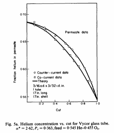
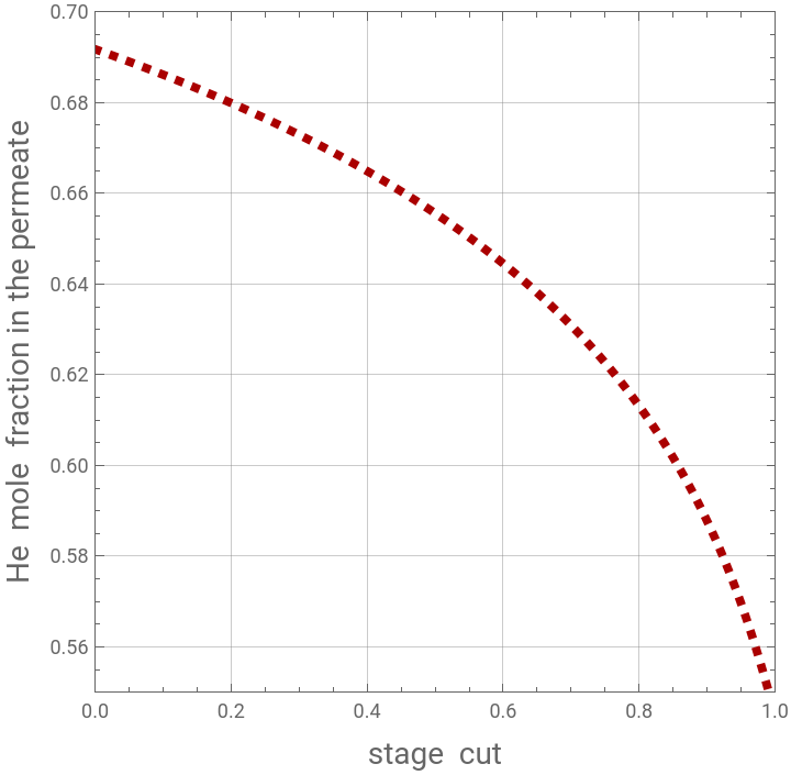
Helium concentration vs. stage cut for Vycor glass tube is given in Fig. 5a of Ref. 1. Parameters are the following : separation factor = 2.62, pressure ratio = 0.363, feed composition = 0.545 He and 0.455 O2. Here, we reproduce Fig. 5a of Ref. 1 using either a co-current or a counter-current gas permeation module and the methodology described in detail in Ref. 2.References:[1] Charles T. Blaisdell, Karl Kammermeyer, Counter-current and co-current gas separation, Chemical Engineering Science, Volume 28, Issue 6, 1973, pp. 1249-1255, https://doi.org/10.1016/0009-2509(73)80077-6[2] H . Binous, U . Zahid and A . Bellagi, Modeling for Multi - component Gas Permeation with Orthogonal Collocation and Arc - Length Continuation, Chemistry Africa (2024) . https://doi .org/10.1007/s42250-024-01167-y
Counter-current Flow Pattern
Counter-current Flow Pattern
In[]:=
eq1i=/()qA(xA[1]-/)/(qB(xB[1]-/));eq2i=+1;=0.545;=0.455;qA=2.62;qB=1;=1.0;=0.363;Np=20;d[0,0]=(2Np^2+1)/6//N;d[Np,Np]=-(2Np^2+1)/6//N;yc[i_]:=Cos[iPi/Np]//N;d[i_,i_]:=-yc[i]/(2(1-yc[i]^2))//N;d[j_,k_]:=If[j≠k&&k≠0&&k≠Np&&j≠0&&j≠Np,(-1)^(j+k)/(yc[j]-yc[k])]//N;d[Np,0]=-1/2(-1)^Np;d[0,Np]=1/2(-1)^Np;d[j_,0]:=If[j≠Np&&j≠0,-1/2(-1)^j/(1-yc[j])];d[j_,Np]:=If[j≠Np&&j≠0,1/2(-1)^(j+Np)/(1+yc[j])];d[0,j_]:=If[j≠Np&&j≠0,2(-1)^j/(1-yc[j])];d[Np,j_]:=If[j≠Np&&j≠0,-2(-1)^(j+Np)/(1+yc[j])];Add=Table[d[i,j]//N,{i,0,Np},{j,0,Np}];xAp[i_]:=2/stAdd[[i,j]]xA[j];yAp[i_]:=2/stAdd[[i,j]]yA[j]xBp[i_]:=2/stAdd[[i,j]]xB[j];xCp[i_]:=2/stAdd[[i,j]]xC[j];yBp[i_]:=2/stAdd[[i,j]]yB[j];qp[i_]:=2/stAdd[[i,j]]q[j];g=0.363;eq1[i_]:=-xAp[i]q[i]qA(xA[i]-/yA[i])-xA[i](qA(xA[i]-/yA[i])+qB(xB[i]-/yB[i]))eq3[i_]:=qp[i]-(qA(xA[i]-/yA[i])+qB(xB[i]-/yB[i]))eq4[i_]:=(1-q[i])yA[i]-q[i]xA[i]yB[i_]:=1-yA[i]xB[i_]:=1-xA[i]xA[Np+1]=;q[Np+1]=;q[1]=(1-theta);unknown=Join[Flatten[Join[Table[{{xA[i],0.5},{yA[i],0.8}},{i,1,Np}],Table[{{q[i],0.6}},{i,2,Np}]],1],{{theta,0.9},{,0.4},{,0.2},{yA[Np+1],0.2}}];sys=Flatten@Join[Table[{eq1[i],eq3[i],eq4[i]},{i,1,Np}],{eq1i,eq2i,yA[Np+1]}];sol=FindRoot[sys/.st1,unknown,MaxIterations100]
y
PAi
y
PBi
p
l
p
h
y
PAi
p
l
p
h
y
PBi
y
PAi
y
PBi
x
fA
x
fB
q
f
p
l
p
h
Np+1
∑
j=1
Np+1
∑
j=1
Np+1
∑
j=1
Np+1
∑
j=1
Np+1
∑
j=1
Np+1
∑
j=1
p
l
p
h
p
l
p
h
p
l
p
h
p
l
p
h
p
l
p
h
x
fA
x
fA
q
f
q
f
q
f
y
PAi
y
PBi
y
PAi
Out[]=
{xA[1]0.0350502,xA[2]0.0384763,xA[3]0.0494378,xA[4]0.0693478,xA[5]0.0990199,xA[6]0.13767,xA[7]0.182855,xA[8]0.231241,xA[9]0.279599,xA[10]0.325463,xA[11]0.3673,xA[12]0.404375,xA[13]0.4365,xA[14]0.46381,xA[15]0.486591,xA[16]0.505182,xA[17]0.519909,xA[18]0.531059,xA[19]0.538859,xA[20]0.543473,yA[2]0.0608359,yA[3]0.0728749,yA[4]0.0940916,yA[5]0.124826,yA[6]0.163957,yA[7]0.208924,yA[8]0.256483,yA[9]0.303601,yA[10]0.34802,yA[11]0.388378,yA[12]0.424047,yA[13]0.454903,yA[14]0.481106,yA[15]0.502951,yA[16]0.520771,yA[17]0.534886,yA[18]0.545571,yA[19]0.553046,yA[20]0.557467,yA[21]0.558931,q[2]0.0306661,q[3]0.0429156,q[4]0.0634504,q[5]0.0925072,q[6]0.130402,q[7]0.177358,q[8]0.233273,q[9]0.297531,q[10]0.368936,q[11]0.445749,q[12]0.525809,q[13]0.606678,q[14]0.685782,q[15]0.760551,q[16]0.828533,q[17]0.887489,q[18]0.935479,q[19]0.970928,q[20]0.992672,theta0.973408,0.0569913,0.943009}
y
PAi
y
PBi
In[]:=
xA[Np+1]=.;xB[Np+1]=.;q[Np+1]=.;q[1]=.;xA[Np+1][s_]:=;q[Np+1][s_]:=;q[1][s_]:=(1-theta[s]);init=Join[Flatten[Table[{xA[i][0](xA[i]/.sol),yA[i][0](yA[i]/.sol)},{i,2,Np}],1],Flatten[Table[q[i][0](q[i]/.sol),{i,2,Np}],1],{xA[1][0](xA[1]/.sol),yA[Np+1][0](yA[Np+1]/.sol),yA[1][0](/.sol),[0](/.sol),[0](/.sol),theta[0](theta/.sol),st[0]1}];initdev=Join[Flatten[Table[{xA[i]'[0]-0.1,yA[i]'[0]-0.1},{i,1,Np}],1],Flatten[Table[{q[i]'[0]-0.1},{i,2,Np}],1],{theta'[0]-0.1,st'[0]-1,'[0]-0.1,'[0]-0.1,yA[Np+1]'[0]-0.1}];aux=Sum[xA[i]'[s]^2+yA[i]'[s]^2,{i,1,Np}]+Sum[q[i]'[s]^2,{i,2,Np}]+theta'[s]^2+st'[s]^2+'[s]^2+'[s]^21;unknown1=Join[Flatten[Table[{xA[i],yA[i]},{i,1,Np}],1],Flatten[Table[q[i],{i,2,Np}],1],{theta,st,,,yA[Np+1]}];
x
fA
q
f
q
f
y
PAi
y
PAi
y
PAi
y
PBi
y
PBi
y
PAi
y
PBi
y
PAi
y
PBi
y
PAi
y
PBi
In[]:=
functions={xA[1]xA[1][s],yA[1]yA[1][s],xA[2]xA[2][s],yA[2]yA[2][s],q[2]q[2][s],xA[3]xA[3][s],yA[3]yA[3][s],q[3]q[3][s],xA[4]xA[4][s],yA[4]yA[4][s],q[4]q[4][s],xA[5]xA[5][s],yA[5]yA[5][s],q[5]q[5][s],xA[6]xA[6][s],yA[6]yA[6][s],q[6]q[6][s],xA[7]xA[7][s],yA[7]yA[7][s],q[7]q[7][s],xA[8]xA[8][s],yA[8]yA[8][s],q[8]q[8][s],xA[9]xA[9][s],yA[9]yA[9][s],q[9]q[9][s],xA[10]xA[10][s],yA[10]yA[10][s],q[10]q[10][s],xA[11]xA[11][s],yA[11]yA[11][s],q[11]q[11][s],xA[12]xA[12][s],yA[12]yA[12][s],q[12]q[12][s],xA[13]xA[13][s],yA[13]yA[13][s],q[13]q[13][s],xA[14]xA[14][s],yA[14]yA[14][s],q[14]q[14][s],xA[15]xA[15][s],yA[15]yA[15][s],q[15]q[15][s],xA[16]xA[16][s],yA[16]yA[16][s],q[16]q[16][s],xA[17]xA[17][s],yA[17]yA[17][s],q[17]q[17][s],xA[18]xA[18][s],yA[18]yA[18][s],q[18]q[18][s],xA[19]xA[19][s],yA[19]yA[19][s],q[19]q[19][s],xA[20]xA[20][s],yA[20]yA[20][s],q[20]q[20][s],thetatheta[s],yA[21]yA[21][s],stst[s],[s],[s]};
y
PAi
y
PAi
y
PBi
y
PBi
In[]:=
Length[sys]
Out[]=
62
In[]:=
SYS=Join[sys/.functions,{aux,yA[1][s]==[s]},init,initdev];SOL=Quiet@NDSolve[SYS,unknown1,{s,-10,10},AccuracyGoal7];
y
PAi
In[]:=
p1=ParametricPlot[{theta[s],yA[Np+1][s]}/.SOL[[1]],{s,-10,5},PlotRange{{0.0,1.0},{0.55,0.70}},FrameTrue,GridLinesAutomatic,AspectRatio1,PlotStyle{Thickness[0.0125],Dashed,Darker@Red},FrameTrue,FrameLabel{Style["stage cut",14],Style["He mole fraction in the permeate",14]},PlotPoints1000]
Out[]=
Co-current Flow Pattern
Co-current Flow Pattern
Comparison between our results and Figure 5a of Ref. 1 indicates close agreement, which provides a validation of the methodology described in Ref. 2.
Comparison between our results and Figure 5a of Ref. 1 indicates close agreement, which provides a validation of the methodology described in Ref. 2.