In this short computational essay, I explore the power of the new functions for Non-Commutative Algebra in the Wolfram Language in the context of quantum mechanics and quantum optics. Given any algebra defined by commutator relations, it is possible to simplify operator expressions systematically. This was shown calculating diverse commutators and Heisenberg picture evolution of well known operators.The recently implemented Baker–Campbell–Hausdorff (BCH) and Zassenhaus formulas are demonstrated through simple yet interesting examples. Potential future applications include exploring time evolution and investigating in depth the properties of Lie algebras.
Please note the following built-in functions on non-commutative algebra needs version 14.3 of Wolfram Mathematica.
Heisenberg picture: commutators and evolution of operators
Heisenberg picture: commutators and evolution of operators
Differential equation for the operator in Heisenberg picture:
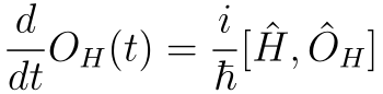
Single mode field
Single mode field
Define scalar variables:
In[]:=
alg=NonCommutativeAlgebra[<|"ScalarVariables"->{h,ω,m}|>];
Hamiltonian for a single mode of radiation :
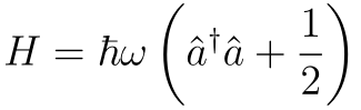
In[]:=
Hsinglemode=hω(**a+1/2);
†
a
Where the annihilation and creation operators hold the commutation relation :
[a,]=1
†
a
In[]:=
commRel=Commutatora,-1;
†
a
h
H,a]
In[]:=
h
†
a
Out[]=
-aω
Hence the differential equation solution is , where the operator at time zero is just the Schrodinger picture annihilation operator
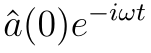
h
[H,]
†
a
In[]:=
h
†
a
†
a
Out[]=
ω
†
a
In this case the solution is
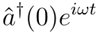
And trivially the number operator commutes with the Hamiltonian:
In[]:=
h
†
a
†
a
Out[]=
0
Position and momentum operators in terms of the ladder operators:
In[]:=
xOp=(a+);pOp=(-a);
h
2mω
†
a
mhω
2
†
a
[H, x]:
In[]:=
NonCommutativePolynomialReduceCommutator[Hsinglemode,xOp],commRel,a,,alg[[-1]]//Simplify
†
a
Out[]=
hω(-a+)
h
mω
†
a
2
We see the term (- + ) appears so can be expressed in terms of momentum operator:
a
†
a
In[]:=
FullSimplify%/.-a+->-p,{m,h,ω}0
†
a
2
mhω
Out[]=
-
hp
m
[H, p] :
In[]:=
NonCommutativePolynomialReduceCommutator[Hsinglemode,pOp],commRel,a,,alg[[-1]]//Simplify
†
a
Out[]=
hω)
hmω
(a+†
a
2
And this one can be expressed in terms of position operator:
In[]:=
FullSimplify%/.a+->x,{m,h,ω}0
†
a
2mω
h
Out[]=
hmx
2
ω
Position and momentum in quantum harmonic oscillator
Position and momentum in quantum harmonic oscillator
Define the algebra and QHO Hamiltonian:
H=+m
2
p
2m
1
2
2
ω
2
x
In[]:=
alg=NonCommutativeAlgebra[<|"ScalarVariables"->{m,ω,h}|>];Hharmonic=+;
p**p
2m
mx**x
2
ω
2
Canonical commutator [x, p] = ℏ :
In[]:=
canonicalCommutator={Commutator[x,p]-h};
/ℏ :
[H,x]
In[]:=
dtx=NonCommutativePolynomialReduce[Commutator[Hharmonic,x],canonicalCommutator,{x,p},alg][[-1]]
h
Out[]=
p
m
/ ℏ :
[H,p]
In[]:=
dtp=NonCommutativePolynomialReduce[Commutator[Hharmonic,p],canonicalCommutator,{x,p},alg][[-1]]
h
Out[]=
-mx
2
ω
We got the same results as before but this time using the algebra of :
xandp
So now we can solve the associated differential equations:
In[]:=
DSolve[{D[x[t],t]==dtx/.p->p[t],D[p[t],t]==dtp/.x->x[t],x[0]==x0,p[0]==p0},{x[t],p[t]},t][[1]]//Simplify//Column
Out[]=
p[t]p0Cos[tω]-mx0ωSin[tω] |
x[t]x0Cos[tω]+ p0Sin[tω] mω |
Baker Campbell Hausdorff and Zassenhaus functions
Baker Campbell Hausdorff and Zassenhaus functions
Resource functions for calculating the nth degree term of Baker Campbell Hausdorff and Zassenhaus expansions:
In[]:=
BCH=ResourceFunction["BakerCampbellHausdorffTerms"]
Out[]=
In[]:=
Zassenhaus=ResourceFunction["ZassenhausTerms"]
Out[]=
Revisiting Heisenberg picture
Revisiting Heisenberg picture
Heisenberg picture operator can also be calculated as , which can be written alternately as . In this form we can use the BCH function (see documentation):
Define the scalar variables:
In[]:=
alg=NonCommutativeAlgebra[<|"ScalarVariables"->{h,ω,t,ϵ}|>];
Calculating the BCH expansion, since we calculated [H, a] before , we use that as a relation for NonCommutativePolynomialReduce :
CollectDSumSimplifyNonCommutativePolynomialReduceBCH,ϵa,,n,NonCommutativeMultiply,{H**a-a**H+aωh},{H,a},alg[[-1]],{n,8},ϵ/.ϵ->0,a
Ht
h
-Ht
h
Recovering the associated function assuming infinite terms, which is clearly an exponential:
Calculating the BCH expansion:
Corresponding closed form of the creation operator:
Interesting closed form cases
Interesting closed form cases
[X, Y] = y Y
[X, Y] = y Y
Van Brunt & Visser Eq.8
[X, Y] = u X + v Y + c I
[X, Y] = u X + v Y + c I
Is not hard to see f(u,v) is a symmetric function:
Van Brunt and Visser Eq.28
We can find a closed form of f(u,u):
Also for f(u, -u):
For this case the generating sequence is:
Quantum Optics: extra commutators and displacement operator
Quantum Optics: extra commutators and displacement operator
Some extra commutators:
Define quadratures:
[X1,X2]:
Non commutative power (so far there is not an automatic simplification for zeroth power):
Test equality for a random sample of integers, and show one of the results:
The GroebnerBasis says the only relation we need is the canonical one, which is expected:
Or we can go the other way around using the BCH formula:
We use again the method that was used for the Heisenberg picture, making the central operator also an exponential:
References
References
◼
Alexander Van-Brunt and Matt Visser 2015 J. Phys. A: Math. Theor. 48 225207
DOI 10.1088/1751-8113/48/22/225207 https://arxiv.org/pdf/1501.02506
DOI 10.1088/1751-8113/48/22/225207 https://arxiv.org/pdf/1501.02506
CITE THIS NOTEBOOK
CITE THIS NOTEBOOK
Exploring non-commutative algebra: commutators, BCH expansion and calculations of bosonic algebra
by Bruno Tenorio
Wolfram Community, STAFF PICKS, August 22, 2025
https://community.wolfram.com/groups/-/m/t/3533713
by Bruno Tenorio
Wolfram Community, STAFF PICKS, August 22, 2025
https://community.wolfram.com/groups/-/m/t/3533713