This notebook series is designed to introduce selected dynamic economic models to both advanced undergraduate and graduate students. Economists have relied on a series of economic models to better understand the otherwise highly complex causal relationship among many economic variables. Dynamic economic models set up by systems of either difference or differential equations are particularly useful in tracing the change in the quantity of unknown economic variables (e.g., the capital stock, demand for labor, aggregate output, etc.) and their interactions over time.
This notebook series aims to help students better understand the depth, usefulness, and limitations of major existing micro and macroeconomic models by demonstrating how we can use Wolfram Mathematica to replicate and reconstruct the core ideas and find dynamic solution of the model.
The model introduced in this notebook series include, among others, (1) the cobweb model of the quantity and price adjustment, (2) Keynes’s aggregate demand model, (3) Hicks’s ISLM model, (4) Samuelson’s investment accelerator model, (5) Kalecki’s investment delay model, (6) the predator-prey interaction model, (7) the epidemic model, (8) Ricardo’s three dimensional business cycle model, (9) Marx-Goodwin business cycle and growth model, (10) Smith’s and Ricardo’s growth model, (11) the Harrod-Domar growth model, (12) the Solow growth model, (13) the RBC model, (14) Romer’s new growth model, and (15) the circuit of capital model.
Introduction
Introduction
The Real Business Cycle (RBC) model is one variant of neoclassical growth models. It shares many assumptions used in Solow’s technology-augmented growth model and of optimal capital stock-consumption growth model proposed by Cass (1965) and Koopmans (1963). Its unique feature lies in its specification of the production technology, or the A-term used in the aggregate production function. The RBC theorists introduce a stochastic term in specifying the A-term, thereby mimicking a certain random changes in the growth process of the capital stock and aggregate output.
In doing so, RBC theorists remove the conventional distinction between the short-run and the long-run, between the business cycle pattern and economic growth process. As the label RBC represents, the dynamic and stochastic variation in the accumulation of the capital stock and aggregate output only comes from the ‘real’ side of the economy (as opposed to monetary side) or from the random and stochastic change in the production technology. Therefore, this approach is often dubbed as ‘non-monetary equilibrium business cycle’ theory.
Following Romer (2011) and Raghavendra and Piiroinen (2023), this note represents the core features of the representative RBC model. Interested readers can also find Snowdon and Vane’s introduction to this school of thought informative (Snowdon and Vane 2005). For an effective presentation, this note intentionally ignores the possible complications associated with households’ optimization behaviors. Instead, the model confines its focus only onto the stochastic change in production technology, the capital stock accumulation, and output growth. A fuller discussion of the representative RBC model requires a certain specification of the behavior of the representative producer and consumer, which introduce a series of additional assumptions such as the firm’s optimization behavior in labor demand and the household’s intertemporal decision over its labor supply, something similar to what we can see in the optimal capital stock-consumption growth model (or neoclassical ‘overlapping generations model’ a la Cass and Koopmans). For our immediate purposes, however, we ignore these representative consumer behaviors in this note.
A stochastic variation in the aggregate output-income and the capital stock per effective worker
A stochastic variation in the aggregate output-income and the capital stock per effective worker
Preliminary note
Preliminary note
The starting point of the RBC model is Solow’s technology-augmented production function. In our previous analysis, we saw that Solow did not explain how the production technology or the A term would change over time. What would happen to the system if the change in A-term is induced by some random shocks that the RBC theorists call ‘stochastic variation.’ How would this stochastic disturbance influence the capital stock per effective labor and the output per effective labor?
The capital stock and aggregate output-income per effective worker
The capital stock and aggregate output-income per effective worker
The intensive form of the capital stock per effective worker and aggregate output-income per effective worker in the RBC model remain the same as in the Cobb-Douglas form of the technology-augmented Solow growth model:
y
α
(A(t)k(t))
k
α
(A(t)k(t))
(
1
)The only difference from Solow’s specification is that the A-term at time t is no longer growing at a constant rate of g, but instead its growth path is affected by a random disturbance.
A
ϵt
(
2
)where ϵ captures this stochastic disturbance.
A static visualization of solution curves with fixed parameters
A static visualization of solution curves with fixed parameters
Let us start by assigning the following arbitrary parameter values and the initial condition for the capital stock per effective labor:
In[]:=
Clear[s,α,δ,n,ϵ,k,k0,y,t,randomWalk,eqn,sol];α=0.5;(*Intensityofcapitalstockpereffectiveworkerinproduction*)s=0.2;(*Thesaveragesavingrate*)δ=0.02;(*Thedepreciationrate*)g=0.01;(*TheconstantgrowthrateofA*)n=0.01;(*Thegrowthrateoflaborforce*)k0=1;(*InitialCapitalStockpereffectiveworker*)
We also generate stochastic disturbance terms, using RandomFunction[GeometricBrownianMotionProcess []] where μ is the mean, σ volatility, and A0 the initial value. Since we need to solve a differential equation, we should convert randomly generated discrete numbers into differential equivalents, using Interpolation[ ]:
μ,σ,A0
In[]:=
seed=1234;SeedRandom[seed];ϵ=RandomFunction[GeometricBrownianMotionProcess[0.01,0.05,1.0],{0,100,0.1}];randomWalk=Interpolation[ϵ["Path"]];eqn={k'[t]==s*((randomWalk[t])*k[t]^α)-(n+g+δ)*k[t],k[0]==k0};sol=NDSolve[eqn,k,{t,0,100}];
The growth of the capital stock is defined as the product of the average saving rate and the output per effective worker. The second terms, (n+g+ δ)k in this definition is what is called ‘break-even’ point in the Solow growth model. Notice that the A-term is now replaced by randomWalk(t) in the capital stock growth equation. In this formulation, we assume that the A-term grows at a constant rate but its growth path is perturbed by the random factor.
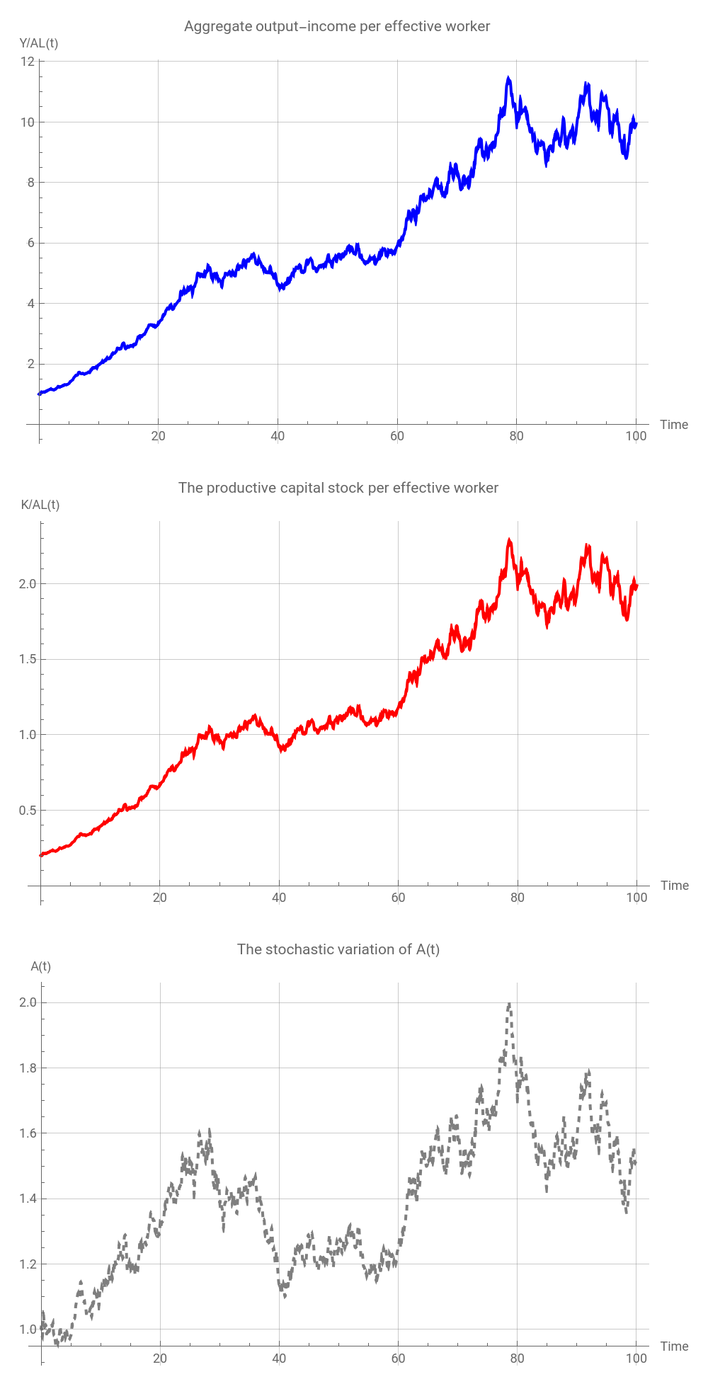
Given these parameter values, the solution curve of aggregate output per effective worker, the capital stock per effective worker, and the very stochastic change in the A-term can be plotted as follow:
In[]:=
GraphicsGrid[{{Plot[(randomWalk[t])*(k[t]/.sol)^α,{t,0,100},PlotLabel->"Aggregate output-income per effective worker",AxesLabel->{"Time","Y/AL(t)"},PlotStyle->Blue,GridLines->Automatic,ImageSize->500]},{Plot[s*(randomWalk[t])*(k[t]/.sol)^α,{t,0,100},PlotLabel->"The productive capital stock per effective worker",AxesLabel->{"Time","K/AL(t)"},PlotStyle->Red,GridLines->Automatic,ImageSize->500]},{Plot[(randomWalk[t]),{t,0,100},PlotLabel->"The stochastic variation of A(t)",AxesLabel->{"Time","A(t)"},PlotStyle->{Gray,Dashed},GridLines->Automatic,ImageSize->500]}},ImageSize->500]
Out[]=
An interactive visualization with varying parameters
An interactive visualization with varying parameters
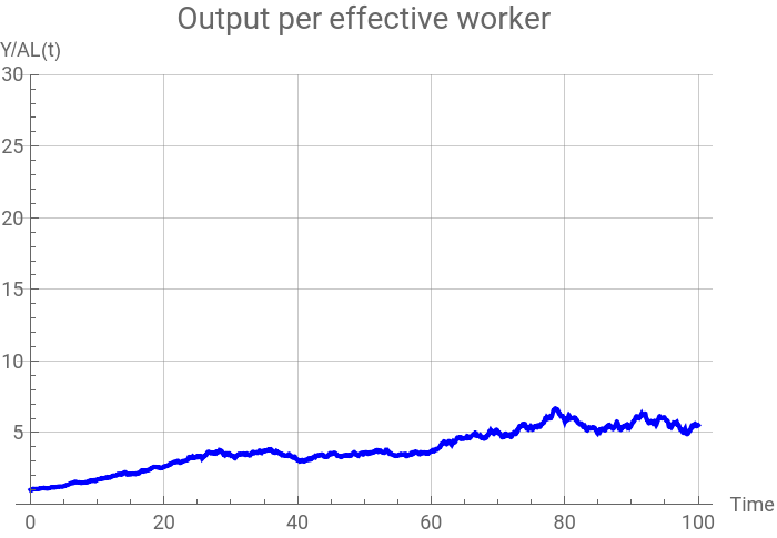
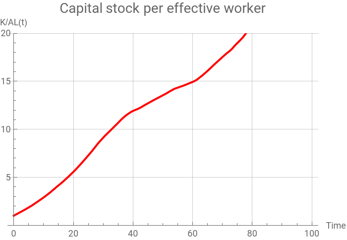
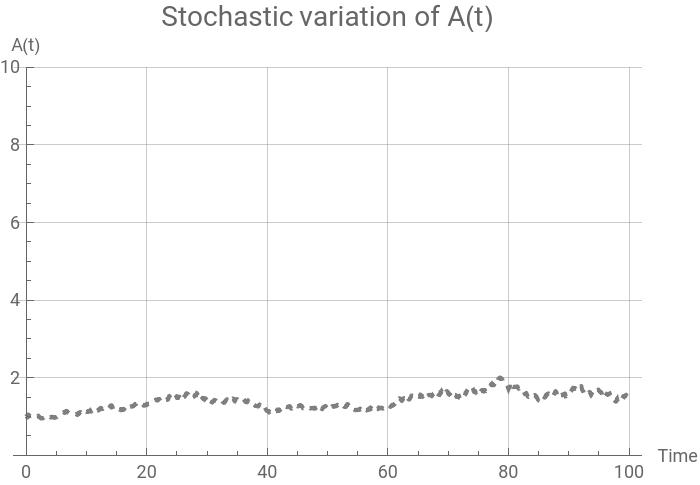
Following the same model structure, we can now create an interactive chart that allows us to see the instantaneous adjustment process in the solution curves by changing crucial parameters. The following syntax does this job:
In[]:=
ClearAll["Global`*"]ManipulateModule{eqn,sol,kSol},eqn={k'[t]==s*((randomWalk[t])*k[t]^α)-(n+δ)*k[t],k[0]==k0};sol=NDSolve[eqn,k,{t,0,100}];kSol=k/.First[sol];RowPlotrandomWalk[t]*(kSol[t]^α),{t,0,100},,PlotkSol[t],{t,0,100},,PlotrandomWalk[t],{t,0,100},,Style["Parameters",Bold],{{s,0.20,"savings rate (s)"},0.1,0.4,Appearance->"Labeled"},{{α,0.4,"intensity of capital (α)"},0.2,0.8,Appearance->"Labeled"},{{δ,0.02,"depreciation rate (δ)"},0.01,0.04,Appearance->"Labeled"},{{g,0.01,"avg. growth rate of A (g)"},0.0,0.1,Appearance->"Labeled"},{{n,0.02,"growth rate of labor force (n)"},0.01,0.05,Appearance->"Labeled"},Delimiter,Button["Want to generate a new stochastic process? Click!",SeedRandom[];path=RandomFunction[GeometricBrownianMotionProcess[0.01,0.05,1.0],{0,100,0.1}];randomWalk=Interpolation[path["Path"]]],ControlPlacement->Top,Initialization:>(k0=1;SeedRandom[1234];path=RandomFunction[GeometricBrownianMotionProcess[0.01,0.05,1.0],{0,100,0.1}];randomWalk=Interpolation[path["Path"]];),SaveDefinitions->True
Out[]=


Conclusion
Conclusion
Compared to Solow’s original growth model, the simulation from this RBC model looks a lot more ‘realistic.’ But this model does not explain where this stochastic term come from and whether this random statistical disturbance can explain large swings in the growth of aggregate output-income. More fundamentally, there is no justification for interpreting the A-term as a proxy of the production technology as we discussed in the previous session. If the stochastic fluctuation persists and if this unanticipated random real factor induces such huge output fluctuations, ironically the classical Marxian ‘class struggle’ theory of income distribution can be equally vindicated by the same narrative.
Reference
Reference
◼
Brian Snowdon and Howard R. Vane, Modern Macroeconomics - Its Origins, Development and Current State, Cheltenham, UK and Northampton, MA, USA: Edward Elgar, 2005, Ch. 6.
◼
David Cass, “Optimal growth in an aggregative model of capital accumulation,” Review of Economic Studies, Vol. 32 (1965), pp.233-240.
◼
David Romer, Advanced Macroeconomics, McGraw-Hill, 2011 (4th edition), Ch. 4.
◼
Srinivas Raghavendra and Petri T. Piiroinen, An Introduction to Economic Dynamics - Modelling, Analysis and Simulation, Routledge: 2023, pp.173-192.
◼
Tjalling C. Koopmans, “On the concept of optimal economic growth,” in The Econometric Approach to Development Planning, Amsterdam: Elsevier, 1963, pp.225-300.
CITE THIS NOTEBOOK
CITE THIS NOTEBOOK
Introduction to dynamic economic models: the real business cycle model
by Hee-Young Shin
Wolfram Community, STAFF PICKS, January 9, 2026
https://community.wolfram.com/groups/-/m/t/3603826
by Hee-Young Shin
Wolfram Community, STAFF PICKS, January 9, 2026
https://community.wolfram.com/groups/-/m/t/3603826