Type II Ternary Liquid Liquid Equilibrium Diagram using Common Tangent Plane
Authors: Housam Binous
Type II Ternary Liquid Liquid Equilibrium Diagram using Common Tangent Plane
Authors: Housam Binous
Authors: Housam Binous
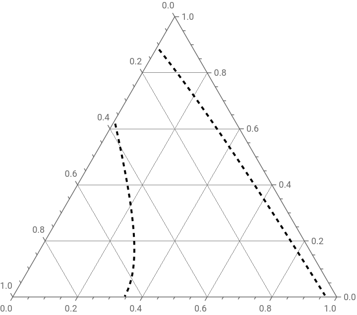
The ternary liquid–liquid equilibrium (LLE) of the methanol–hexane–heptane system was calculated using the NRTL activity-coefficient model through two independent numerical approaches: the common tangent method and the arc-length continuation method. The resulting binodal curves obtained from both techniques are plotted together in the ternary composition diagram.
The common tangent method determines pairs of equilibrium compositions by satisfying the tangent-plane criterion on the Gibbs free energy of mixing surface, while the arc-length continuation method directly follows the solution branch of the phase-equilibrium equations using a continuation parameter. These complementary approaches enable accurate determination of the liquid–liquid coexistence boundary over the entire heterogeneous region.
The calculated phase diagram exhibits Type-II ternary liquid–liquid equilibrium behavior, characterized by a partially miscible binary pair (methanol–hexane) and a third component (heptane) that remains completely miscible with one of the binary constituents. Consequently, the binodal curve intersects the methanol–hexane side of the ternary diagram and extends into the interior of the composition space, forming the characteristic open miscibility gap associated with Type-II systems.
As shown in the figure, the coexistence curves predicted by the common tangent and arc-length continuation methods overlap almost perfectly throughout the heterogeneous region. The excellent agreement between the two independently implemented numerical procedures confirms the correctness of the NRTL model calculations and demonstrates the reliability of both methods for predicting ternary liquid–liquid equilibria.
Overall, the comparison reveals that the common tangent and arc-length continuation methods provide essentially identical descriptions of the Type-II phase behavior of the methanol–hexane–heptane system, with negligible deviations in the predicted binodal boundary and critical solution region. This agreement validates both the thermodynamic model and the numerical algorithms employed in the present work.
Method based on common tangent plane
Computing Tie lines and LLE curve
Hexane = component 1
Heptane = component 2
Methanol = component 3
Hexane = component 1
Heptane = component 2
Methanol = component 3
In[]:=
ClearAll["Global`*"];R=1.9872041;(*universalgasconstant*)T=273.15+32.85;(*temperature*)(*NRTLPARAMETERS*)a13=0.42399900;a12=0.301800;a32=0.440800;t31=1287.78000;t13=1915.07700;t23=1598.3120000;t32=1566.43700;t12=-285.9411;t21=252.997600;α={{0.,a12,a13},{a12,0.,a32},{a13,a32,0.}};τ={{0.,t12,t13},{t21,0.,t23},{t31,t32,0.}}/(RT);
In[]:=
α//MatrixForm
Out[]//MatrixForm=
0. | 0.3018 | 0.423999 |
0.3018 | 0. | 0.4408 |
0.423999 | 0.4408 | 0. |
In[]:=
τ//MatrixForm
Out[]//MatrixForm=
0. | -0.470233 | 3.14936 |
0.416057 | 0. | 2.62844 |
2.11777 | 2.57602 | 0. |
In[]:=
G[i_,j_]:=Exp[-α[[i,j]]τ[[i,j]]];(*COMPOSITIONVECTOR*)xvec[x1_,x2_]:={x1,x2,1-x1-x2};(*NRTLACTIVITYCOEFFICIENTS*)lnGamma[i_,x1_,x2_]:=Module[{x,term1,term2},x=xvec[x1,x2];term1=Sum[x[[j]]τ[[j,i]]G[j,i],{j,1,3}]/Sum[x[[k]]G[k,i],{k,1,3}];term2=Sum[x[[j]]G[i,j]/Sum[x[[k]]G[k,j],{k,1,3}](τ[[i,j]]-Sum[x[[m]]τ[[m,j]]G[m,j],{m,1,3}]/Sum[x[[m]]G[m,j],{m,1,3}]),{j,1,3}];term1+term2];gamma[i_,x1_,x2_]:=Exp[lnGamma[i,x1,x2]];(*DIMENSIONLESSGIBBSENERGYOFMIXING:g/RT*)gmix[x1_,x2_]:=Module[{x},x=xvec[x1,x2];Sum[x[[i]]Log[x[[i]]],{i,1,3}]+Sum[x[[i]]lnGamma[i,x1,x2],{i,1,3}]];(*DERIVATIVES*)dgdx1[x1_,x2_]:=Evaluate[D[gmix[u,v],u]/.{u->x1,v->x2}];dgdx2[x1_,x2_]:=Evaluate[D[gmix[u,v],v]/.{u->x1,v->x2}];(*UNKNOWNS*)vars={x1a,x2a,x1b,x2b,m1,m2};(*COMMONTANGENTEQUATIONS*)eq1=dgdx1[x1a,x2a]==m1;eq2=dgdx1[x1b,x2b]==m1;eq3=dgdx2[x1a,x2a]==m2;eq4=dgdx2[x1b,x2b]==m2;eq5=gmix[x1b,x2b]-gmix[x1a,x2a]==m1(x1b-x1a)+m2(x2b-x2a);(*EXTRACONSTRAINT-Preventtrivialsolutionxα=xβ*)eq6=(x1b-x1a)^2+(x2b-x2a)^2==d;
In[]:=
(*firstrangefordvalues---verysmalld=0.001yieldapproximatelytheplaitpoint*)d0t=Table[i,{i,0.07,0.085,0.001}];
In[]:=
(*solution*)solct=Table[FindRoot[{eq1,eq2,eq3,eq4,eq5,eq6/.d->d0t[[i]]},{{x1a,0.33},{x2a,0.4},{x1b,0.060},{x2b,0.4},{m1,-0.65},{m2,-0.45}},MaxIterations->1000],{i,1,Length@d0t}];

In[]:=
(*secondrangefordvalues*)d0t=Table[i,{i,0.085,0.30,0.001}];
In[]:=
(*solution*)solct1=Table[FindRoot[{eq1,eq2,eq3,eq4,eq5,eq6/.d->d0t[[i]]},{{x1a,0.31},{x2a,0.61},{x1b,0.18},{x2b,0.35},{m1,-1.05},{m2,-0.38}},MaxIterations->1000],{i,1,Length@d0t}];
In[]:=
(*thirdrangefordvalues*)d0t=Table[i,{i,0.3,0.38,0.001}];
In[]:=
(*solution*)solct3=Table[FindRoot[{eq1,eq2,eq3,eq4,eq5,eq6/.d->d0t[[i]]},{{x1a,0.88},{x2a,0.076},{x1b,0.34},{x2b,0.028},{m1,-0.004},{m2,-2.58}},MaxIterations->1000],{i,1,Length@d0t}];
In[]:=
solctf=Join[solct,solct1,solct3];
In[]:=
DATA1ct=Table[{x1a,x2a,1-x1a-x2a}/.solctf[[i]],{i,1,Length@solctf}];DATA2ct=Table[{x1b,x2b,1-x1b-x2b}/.solctf[[i]],{i,1,Length@solctf}];
Type II liquid - liquid equilibrium (LLE) diagram
In[]:=
p1=Show[TernaryListPlot[{DATA1ct,DATA2ct},Joined->True,GridLines->Automatic,PlotRange->All,PlotStyle->{{Black,Dashed,Thick},{Black,Dashed,Thick}}]]
Out[]=
Method based on arc - length
In[]:=
In[]:=
K={GAMMA1/GAMMA1p,GAMMA2/GAMMA2p,GAMMA3/GAMMA3p}/.x31-x1-x2/.xp31-xp1-xp2;
In[]:=
z={0.5,0.1,0.4};sol=FindRoot(K[[i]]-1)z[[i]](1+(K[[i]]-1)ϕ)0,x1z[[1]](1+(K[[1]]-1)ϕ),x2z[[2]](1+(K[[2]]-1)ϕ),xp1K[[1]]z[[1]](1+(K[[1]]-1)ϕ),xp2K[[2]]z[[2]](1+(K[[2]]-1)ϕ),{ϕ,0.1,0.9},{x2,0.3,0.40},{x1,0.1,0.2},{xp1,0.6,0.7},{xp2,0.25,0.3},MaxIterations10000
3
∑
i=1
Out[]=
{ϕ0.358168,x20.0659417,x10.333295,xp10.798733,xp20.161032}
In[]:=
z={0.5,a,1-0.5-a}/.aa[s];
In[]:=
eq1=(K[[i]]-1)z[[i]]/(1+(K[[i]]-1)ϕ)0/.x1x1[s]/.x2x2[s]/.xp1xp1[s]/.xp2xp2[s]/.ϕϕ[s];eq2=x1z[[1]]/(1+(K[[1]]-1)ϕ)/.x1x1[s]/.x2x2[s]/.xp1xp1[s]/.xp2xp2[s]/.ϕϕ[s];eq3=x2z[[2]]/(1+(K[[2]]-1)ϕ)/.x1x1[s]/.x2x2[s]/.xp1xp1[s]/.xp2xp2[s]/.ϕϕ[s];eq4=xp1K[[1]]z[[1]]/(1+(K[[1]]-1)ϕ)/.x1x1[s]/.x2x2[s]/.xp1xp1[s]/.xp2xp2[s]/.ϕϕ[s];eq5=xp2K[[2]]z[[2]]/(1+(K[[2]]-1)ϕ)/.x1x1[s]/.x2x2[s]/.xp1xp1[s]/.xp2xp2[s]/.ϕϕ[s];eq6=x1'[s]^2+x2'[s]^2+xp1'[s]^2+xp2'[s]^2+ϕ'[s]^2+a'[s]^21;derivinit={x1'[0]0,x2'[0]0,xp1'[0]0,xp2'[0]0,ϕ'[0]1,a'[0]-0.2};init={x1[0](x1/.sol),x2[0](x2/.sol),xp1[0](xp1/.sol),xp2[0](xp2/.sol),ϕ[0](ϕ/.sol),a[0]0.05};
3
∑
i=1
In[]:=
system=Flatten[Join[{{eq1,eq2,eq3,eq4,eq5,eq6},derivinit,init}]];