Abstract: When viewing a “quantum Boolean function” as a unitary matrix , constructed from a pre-defined set of gates such as {Hadamard,S,T,Pauli X, Pauli Y, Pauli Z}, it is clear that as the permitted number of gates in the circuit increases, the number of points reachable in the Bloch sphere (given a fixed initial pure state input) should also increase. In the following discussion, I study the empirical relationship between the gate complexity of the circuit and the number of reachable points in the Bloch sphere.
n
2
n
2
Motivation
In classical computer science, a Boolean circuits with n input bits is a directed acyclic graph in which every node there exists either an AND gate, an OR gate, or a NOT gate. One of these gates is designated as the output gate. Such a circuit naturally computes a function of its n inputs. [1] So, essentially, a Boolean circuit is equivalent to a Boolean function. In general, complexity quantifies the resources required to implement a computation. For example, a Boolean function’s complexity can be defined as the minimal number of gates, chosen from a given gate set, necessary to evaluate the function. [2]
The question also translates to quantum circuits. If you started making progressively more complex quantum circuits, starting from one gate, then two gates etc, you could look at all possible quantum circuits, made from some discrete set of gates. Then one can ask, how complicated are function that can be produced from that set of quantum gates. One way to characterize that, would be to ignore all the output wires, except for one, and then color a Bloch sphere based on the values that come out of that one wire, and then examine how does the change in complexity of the quantum circuit affect the colouring of the Bloch sphere.
Quantum computational complexity is rooted in circuit complexity. However, quantum complexity is also related to the phases of matter, holography in high-energy physics, in the context of the anti-de-Sitter-space/conformal field-theory (AdS/CFT) correspondence, and the event horizon of black holes. [2]
Strategy
Strategy
Bloch Sphere
Bloch Sphere
In quantum mechanics and computing, the Bloch sphere is a geometrical representation of the state space of a two-level quantum mechanical system, called qubit [3]. It was originally used for pure states, which are states the can be mathematically represented by a single ket vector [4]. However, one can generalize the Bloch sphere in order to represent mixed states as well. Mixed states are essentially statistical ensembles of pure states [5]. The difference between the vectors of pure and mixed states is that pure states are mapped on the surface of the Bloch sphere, while mixed states occupy the space inside the sphere.
Gate Enumeration
Gate Enumeration
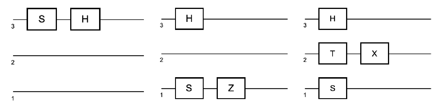
The process of gate enumeration is the process of making progressively more complex circuits by a composing a set of gates. First, we begin by creating circuits that contain only one gate, which can be placed at any wire. (For bipartite systems we have 2 wires, while for tripartite systems we have three). This gate can be any one from the discrete set {S, T, Pauli X, Pauli Y, Pauli Z, Hadamard}. Then we create circuits by composing any two quantum gates either sequentially or in parallel. So, two examples of such circuits are: Then we do the same with three, four and maybe 5 gates, although the notebook’s rendering time increases exponentially.
Mapping the Circuits in the Bloch Sphere
Mapping the Circuits in the Bloch Sphere
For each produced circuit, we apply the corresponding operator to the pure input state and we get an output state. Then we partially trace over all the wires except for one (we choose wire #1). The result will generally be a mixed state, and we map it inside the Bloch sphere. Many points from different circuits coincide. We colour the points based on their multiplicity, from red, corresponding to relatively few, to green, which corresponds to relatively many. Thus, the greener points are easier to get to, because they represent more equivalent circuits, and by equivalent circuits we mean that they reach the same reduced state in wire #1.
Code
Code
Bloch Sphere Code
Bloch Sphere Code
Circuits Code
Circuits Code
Gate Enumeration Code
Gate Enumeration Code
Non-Entangled Bipartite Systems
Non-Entangled Bipartite Systems
The first case of circuit we examine is a circuit with two wires, that receives a non-entangled bipartite system as an input. For this purpose, we create this state by taking the tensor product of two random qubits.
Qubit11=ResourceFunction["QuantumDiscreteState"][{-0.053474485320397516-0.6991870497253331 I,0.5855969423888849-0.4066376396509459 I}];Qubit12=ResourceFunction["QuantumDiscreteState"][{0.6511383417897777+0.24372022239416802 I,0.41299386259852816-0.588264721450593 I}];InputState1=ResourceFunction["QuantumTensorProduct"][Qubit11,Qubit12];Print["Entangled:",ResourceFunction["QuantumEntangledQ"][InputState1,{{1},{2}}]]
Entangled:False
Then, following the aforementioned tactic, we print the output states we get from the wire #1
Points1=CalculateCircuitPoints[InputState1,4];//AbsoluteTiming
Number of different non-equivalent circuits for progressively larger number of gates: {7,24,65,143,0}
Out[]=
{308.803,Null}
PrintCircuitPoints[Points1]

Out[]=
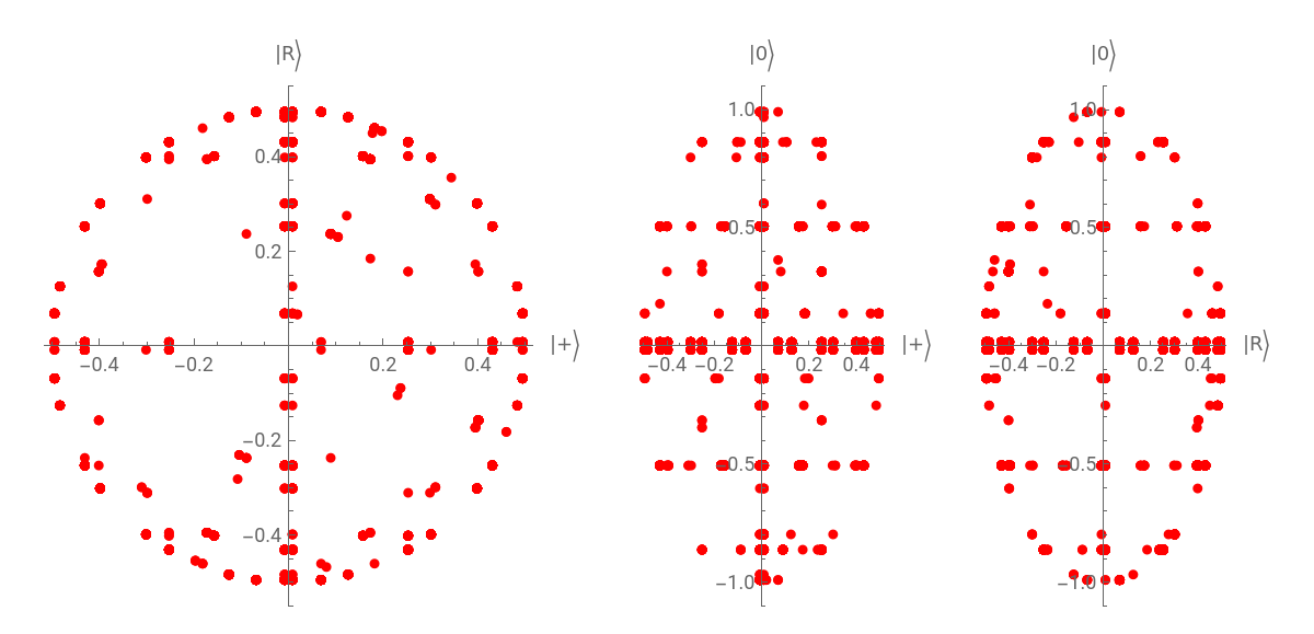
We notice that, while we start form non-entangled state and the circuits do not alter the concurrence monotone of the subsystems 1 and 2, after the partial trace, in general, we still end up with a mixed state which lies inside the Bloch sphere. The result does not depend on whether the gates are composed sequentially or in parallel. (We know that the concurrence monotone is not increased by utilizing the commented out code in Circuit Code, which has been commented out for rendering speed purposes.)
Entangled Bipartite System
Entangled Bipartite System
We follow the same process for circuits with different complexities that receive a random entangled bipartite system as an input state.
InputState2=ResourceFunction["QuantumDiscreteState"][{-0.22446682730322437`-0.466111006924916` ,-0.07522345075488936`-0.4597275598228936` ,0.06975156663871795`-0.6003440557182724` ,0.3845265302755939`-0.04699209602766014` }];Print["Entangled: ",ResourceFunction["QuantumEntangledQ"][InputState2,{{1},{2}}]]
Entangled: True
Points2=CalculateCircuitPoints[InputState2,4];//AbsoluteTiming
Number of different non-equivalent circuits for progressively larger number of gates: {7,24,64,136,0}
Out[]=
{258.469,Null}
PrintCircuitPoints[Points2]

Entangled Tripartite System
Entangled Tripartite System
Now, we do the same job with a random entangled tripartite system.
Concluding remarks
Concluding remarks
In this project we have reached the following conclusions:
◼
The distribution states that we get from a single specific wire out of the circuits composed from any combination of gates from the discrete set {Hadamard,S,T,Pauli X, Pauli Y, Pauli Z} is not random, but seem to lie on something akin to ellipsoids.
◼
There are states which are represented by a larger number of equivalent circuits. That means, that these states are easier to get to.
◼
Circuits that lead to the same states (or, else, points in the Bloch sphere) from wire 1 are equivalent. The number of different non-equivalent circuits we get from the composition of the aforementioned gates increases with similar rate when we increase the number of gates, either when we have bipartite or tripartite system.
◼
While we start form non-entangled state and the circuits do not alter the concurrence monotone of the subsystems 1 and the rest, after the partial trace, in general, we still end up with a mixed state which lies inside the Bloch sphere. The result does not depend on whether the gates are composed sequentially or in parallel.
Keywords
Keywords
◼
Quantum Gate Complexity
◼
Quantum Circuits
◼
Quantum Information
◼
Bloch Sphere
Acknowledgment
Acknowledgment
First, I would like to thank Stephen Wolfram for assigning to me a project suitable to my interests. Also, I would like to thank my mentor Tobias Canavesi for his suggestions on the code, Hatem Elshatlawy for checking my notebook and, Jesse Friedman who answered to all my questions regarding the Wolfram Language.
References
References
◼
[2] Jonas Haferkamp, Philippe Faist, Naga B. T. Kothakonda, Jens Eisert, and Nicole Yunger Halpern, “Linear growth of quantum circuit complexity. https://arxiv.org/pdf/2106.05305.pdf