Wolfram Cloud Document

The aim of this project is to give intuitive insight into the elusive nature of a gas contained in a box through the use of the kinematic approach.

We investigate the dynamics of a 1D hard-sphere system, also referred to as a hard-rod gas. By employing the event-driven simulation method, we compute the evolution of a system of colliding particles and visualize the properties of the model. We model a container with two species of gas particles separated by a wall and explore the dependency on relevant parameters.

1. Hard Spheres

1.1. Introduction and setup

1.1.1. Details of the model

The system of interest will be a 1-dimensional container filled will particles, exhibiting behaviour of a gas. To be exact, the particles will be modelled as hard spheres, that is, described by the following interaction potential (with σ being the radius of the particle):

u(x) =



∞	0 < x <= σ
0	x > σ

,which conveys the key idea, that the particles in this model do not repel or attract each other, but collide at direct contact.Now, imagine the same gas-filled container divided in the middle by a movable wall, or a piston, reacting to the impacts of particles on both sides. The particles in the left side of the container will be referred to as species α, or A, and the particles to the right as species β, or B. The two species can have different properties, come into contact and interact directly, or be separated by a wall-particle, mediating the interactions. We should keep in mind, that in a 1D hard-sphere gas only adjacent particles can collide, and no particles can pass through each other. In other words, the particles are in a fixed order.

1.1.2. Coding the simulation

The core of our approach at the solution is the event-driven method of simulation. Instead of solving for the positions and velocities of particles every fixed timestep, we are going to compute the time until all possible future collisions for given initial conditions, and then evolve the system analytically up to that point. Notably, this means, that each timestep of an event-driven simulation is of different length. This realisation of the simulation allows for faster computation, and, in some cases, avoiding numerical errors.

Below, we include relevant secondary functions, necessary to compute a timestep of a simulation successfully.

Time until a collision between two given particles is handled by the function given below:

In[]:=

CollisionTime[x1_,x2_,v1_,v2_,r1_,r2_]:=Module[{Δx,Δv,Δt,d},d=r1+r2;Δv=v2-v1;Δx=x2-x1;Δt=If[ΔvΔx>=0,Infinity,

-(ΔvΔx+Sqrt[

Δv

])

Δv

]];

Update of the position of a particle with a constant velocity is simply:

In[]:=

Move[x_,v_,t_]:=Module[{},x+tv];

To realise a collision, we need a function that will compute the final velocities of colliding particles. We implement it as follows:

In[]:=

doCollision[x1_,x2_,v1_,v2_,r1_,r2_,m1_,m2_]:=Module[{Δx,Δv,v1New,v2New},Δv=v2-v1;Δx=x2-x1;v1New=v1+

2m2

m1+m2

Δv;v2New=v2-

2m1

m1+m2

Δv;{v1New,v2New}];

Below we introduce the master function for the simulation of a hard-sphere gas. It allows us to model two different particle species separated by a wall-particle. It also contains the implementation of a spring-wall, which will be discussed later. ⟶ HSsim[] (see: Code appendix) The code for this function (and other function, which take up a lot of space) is included in the Code appendix, at the end of the post.

1.2. Numerical experiments

1.2.1. Setup

Having constructed the hard-sphere model framework, we can finally run proper simulations. While we might start with an example with particles of one species bouncing around in a box, the goal is to simulate two species separated by a wall.

For the case with a wall-particle, there are two approaches that come to mind: a lightweight wall, that is going to act as a probe at the interface between two gases, or a heavy wall, which will posses its own significant momentum, and will influence the dynamics of the system.

In the following sections we present examples of system evolution for these two approaches.

For all cases in this section, unless specified otherwise, the simulation parameters are as follows (these will be referred to as standard parameters):

In[]:=

nA=1;nW=0;nB=1;RA=5;RW=20;RB=5;width=100;vmax=10;mA=1;mW=

;mB=1;wallSpring=False;springConst=1;steps=10;

Now we can construct an input list, which will be then passed to the master function:

In[]:=

input:=<|"PosAlpha"->Table[{2RA+3RA(i-1)},{i,1,nA}],"PosWall"->Table[{width/2+2RW(i-1)},{i,1,nW}],"PosBeta"->Reverse[Table[{width-2RB-3RB(i-1)},{i,1,nB}]],"VelAlpha"->Table[{vmax},{i,1,nA}],"VelWall"->Table[{0},nW],"VelBeta"->Table[{vmax},{i,1,nB}],"AlphaRadius"->RA,"WallRadius"->RW,"BetaRadius"->RB,"MassAlpha"->mA,"MassWall"->mW,"MassBeta"->mB,"Steps"->steps,"BoxWidth"->width,"SpringConst"->springConst,"WallSpring"->wallSpring|>

The function used to plot the trajectories of particles is defined as follows: ⟶

PlotEvolution[]

(see: Code appendix)

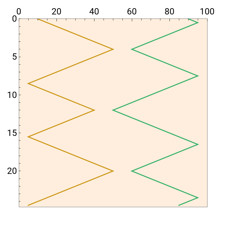
Now, we can finally simulate the evolution of a simple, two-particle system:

In[]:=

simulationResult=HSsim[input];

...and plot the result of the simulation. The particle trajectories are colored randomly, to be distinguishable more easily:

In[]:=

PlotEvolution[simulationResult]

Out[]=

In the plot above, the initial state is at the top, and the system evolves in time along the vertical axis. We can also consider a system with one heavy wall (portrayed by the gray line), and a few more particles on each side, while also making the box a bit wider (note the greater radius of the wall-particle):

We can now expand our simulation to a greater number of particles. The purpose of giving the particles the same initial velocities is to eventually observe how they evolve into disorder.

Clearly, the core of our interest will be much longer simulations, where we can see both the desired disorder and the interesting behavior of the wall-particle:

1.2.2. Energy conservation plots

One of the collective properties of the system, which we can easily extract from the simulation is kinetic energy of each of the components. After all, we track the evolution of velocities of every particle in the simulation. By combining this data, we will be able to see how the energy is transferred during collisions, but also check if the total energy is conserved (which it ought to be, if the simulation works as expected).

The motion of the wall is periodic, which has been cross-checked in numerous simulations spanning across wide range of parameters (results of longer simulations weight much more). We will make use of this fact in following sections.

1.2.3. Varying the radius

Final fit of the model to the simulation data:

1.2.4. The appearance of power law

Final fit of the model to the simulation data:

Although interesting, the theoretical foundations of this relation, and the one found in the previous section, will not be explored further in this simulation-oriented post.

1.2.5. Asymmetric case

Up to this point, we considered particles of the same kind on both sides of the wall. The framework allows us, however, to choose the parameters of both gasses separately. Below, we consider an asymmetric case with a lightweight wall-particle, acting as a probe between two gas species.

Here, we give an example of a setup of an asymmetric simulation:

We can also take a look at the energy and wall position plots:

Due to the use of the lightweight wall approach, the behaviour of the wall-particle is much more erratic, however, periodic motion can still be observed. In principle, tracking its position allows us to see the asymmetric system reaching an equilibrium.

1.3. Extracting the Equation of State

1.3.1. Virial expansion

1.3.2. Comparing theory and simulation

1.4. Adding a spring to the wall

This section is devoted to modelling the wall-particle as a harmonic oscillator. Initially, the particle will reside in the minimum of a harmonic potential, and every collision with adjacent gas-particles will cause it to oscillate around the position of equilibrium.

1.4.1. Setting up the simulation

Part of the code has been already implemented in the master function introduced at the beginning, but there are several crucial functions left to be defined.

Time until a collision between a gas particles and a spring-wall-particle requires a slightly more involved function:

To update the position of the wall, we need a solution for the harmonic oscillator. Just for the purpose of visualization, we may compute additional positions along the way (useful especially with few particles, and hence – few collision timesteps). The function handling the update should also return the final velocity of the wall-particle. All that results in the following function:

1.4.2. Example results

Let us run a simple simulation to test the newly introduced spring-wall functionality:

...and plot the result:

Now we can plot the kinetic energies of the components of the system. The sharp changes in the kinetic energy of the oscillating wall are not physical, and are a result of lesser number of global timesteps of the simulation:

As we should expect, total kinetic energy is not conserved – it is partially stored in the deformed spring, in the form of potential energy. We can clearly see the regions of harmonic motion and the points of collision with a gas-particle.

We are in the process of analysing this simulation functionality further. Many other numerical experiments can be performed, which a curious reader is also encouraged to try.

Concluding Remarks

As we have shown, even the simplest 1-dimensional model of a gas has a lot to offer in terms of arising complexity, programming challenges and physics that we can extract from it.

In terms of outlook for the future, there is certainly a lot more to experiment on. We can, for instance, model a solid wall as a lattice of masses connected by springs – code for which is already partially done. We can then place such a wall in a container, separating two gasses, similarly to what has been shown above. An extension of the hard-sphere event-driven simulation to 2D case is also possible, but, due to additional complexity (both model-wise and code-wise) it deserves its own separate project.

Acknowledgments

I want to express my gratitude to my team from the International Physicists’ Tournament – I wouldn’t be a part of this summer school without them. I would also like to thank the dean of student affairs at my faculty, Krzysztof Turzyński, who made the participation in the WSS2024 possible. Lastly, I want to acknowledge Stephen Wolfram for suggesting the idea for this interesting project.

References

Stephen Wolfram (2023), “Computational Foundations for the Second Law of Thermodynamics,” Stephen Wolfram Writings. writings.stephenwolfram.com/2023/02/computational-foundations-for-the-second-law-of-thermodynamics.

Cite This Notebook

“Particles in a box: Kinetic Gas Theory and simulations”
by Jakub Trzaska
https://community.wolfram.com/groups/-/m/t/3210337