CITE THIS NOTEBOOK: Characterizing Coarse Graining with Causal Graphs by Hanfeng Zhai. Wolfram Community JAN 13 2023.
Abstract
Causal graphs are ubiquitous as a powerful tool for representing natural and engineered systems, including systems like molecular dynamics, particle and planetary collisions, chemical reactions, etc. Generally speaking, the higher the order, the higher the computational burden is required. In many engineering applications, scaling up the computation to capture the exact system is crucial. A crucial step is to reduce the order of the system with minimal loss of information, by performing a kind of coarse-graining procedure. In this project, we aim to understand and characterize coarse-graining as order reduction for hard sphere gas systems and develop a coarse-grained model for the causal graph derived from particle collision systems. We first examine the properties of spatial coarse-graining by testing various physical properties including density distribution, collision rate, kinetic energy, etc., and further examine their causal graphs by analyzing their adjacency matrices, motifs distributions, etc. We show that under ideal gas law, the proposed coarse-graining models are shown to be consistent in collision rate. We also propose a new method to do temporal coarse-graining on causal graphs retaining the same collision rate and test their motifs and related causal graph statistics. Our work sheds light on multiscale modeling and brings in a deeper understanding of coarse-graining by employing graph-based models.
Causal graphs are ubiquitous as a powerful tool for representing natural and engineered systems, including systems like molecular dynamics, particle and planetary collisions, chemical reactions, etc. Generally speaking, the higher the order, the higher the computational burden is required. In many engineering applications, scaling up the computation to capture the exact system is crucial. A crucial step is to reduce the order of the system with minimal loss of information, by performing a kind of coarse-graining procedure. In this project, we aim to understand and characterize coarse-graining as order reduction for hard sphere gas systems and develop a coarse-grained model for the causal graph derived from particle collision systems. We first examine the properties of spatial coarse-graining by testing various physical properties including density distribution, collision rate, kinetic energy, etc., and further examine their causal graphs by analyzing their adjacency matrices, motifs distributions, etc. We show that under ideal gas law, the proposed coarse-graining models are shown to be consistent in collision rate. We also propose a new method to do temporal coarse-graining on causal graphs retaining the same collision rate and test their motifs and related causal graph statistics. Our work sheds light on multiscale modeling and brings in a deeper understanding of coarse-graining by employing graph-based models.
Spatial Coarse-Graining for Macro-dynamics
Spatial Coarse-Graining for Macro-dynamics
Spatial Coarse-Grain: Survey and Formulation
Spatial Coarse-Grain: Survey and Formulation
For decades, a key problem in computational engineering is the bridge of multiple scales, i.e. multiscale modeling. Physically, considering the length scale in the real world, this stands for bridging over Ångström, nanometers, micrometers, meters, etc. Mathematically and numerically, this could mean bridging different scales of order. Multiscale modeling includes bottom-up and top-down approaches. In bottom-up approaches, particle-based simulations are usually the fundamental approach. A central method employed for particle simulations is coarse-graining, i.e., reducing the order of the systems by assuming multiple smaller particles constitute a larger particle (Figure 1).
Figure1:SchematicofSpatialCoarse-Graining.
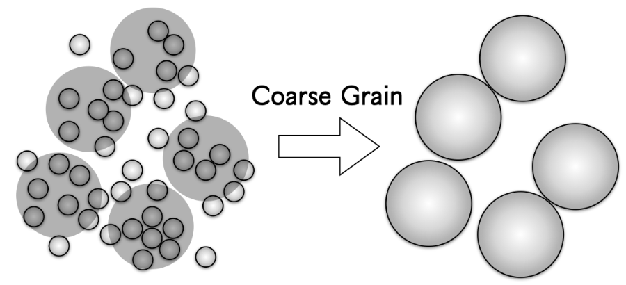
Such a simple and intuitive approach has been widely adopted in many scientific communities in molecular modeling, computational biology, granular flow, and many others. If one does not assume a new inter-particular forcefield, the hierarchical structure of the microscale particular structure is not preserved, making such a coarse-graining approach not feasible in problems like solid mechanics, soft materials, etc. However, if one is curious about the flow dynamics or thermodynamics of the gas state, just resizing the particle and rearranging the numbers with the same forcefield may also be considered as a way of coarse-graining. Such a method has been widely used in granular flows to study the morphology of multiphase systems that are widely used in 3D printing, manufacturing, etc. Our coarse-graining assumptions are mainly inspired by the work in discrete element simulations [Lu et al., 2016; Widartiningsih et al., 2020; Kanjilal & Schneiderbauer, 2021].
Here, we adopt such systems and examine the coarse-graining methods in the case of gas dynamics, curious about three core questions: (1) Can this coarse-graining approach (order reduction) be applied to hard sphere gas systems? (2) If the answer to (1) is Yes, what are the feasibility and limitations of such an approach? (3) What are the hidden mechanism of such coarse-graining and can we bring in a deeper understanding with the Wolfram Physics Project? To answer these questions, we begin by carrying out examine the global and local dynamics of different coarse-grained systems, and strive to understand the systems with causal graphs.
Here, we adopt such systems and examine the coarse-graining methods in the case of gas dynamics, curious about three core questions: (1) Can this coarse-graining approach (order reduction) be applied to hard sphere gas systems? (2) If the answer to (1) is Yes, what are the feasibility and limitations of such an approach? (3) What are the hidden mechanism of such coarse-graining and can we bring in a deeper understanding with the Wolfram Physics Project? To answer these questions, we begin by carrying out examine the global and local dynamics of different coarse-grained systems, and strive to understand the systems with causal graphs.
Macroscale Dynamics: An Illustrative Case
Macroscale Dynamics: An Illustrative Case
Overall Dynamics
Overall Dynamics
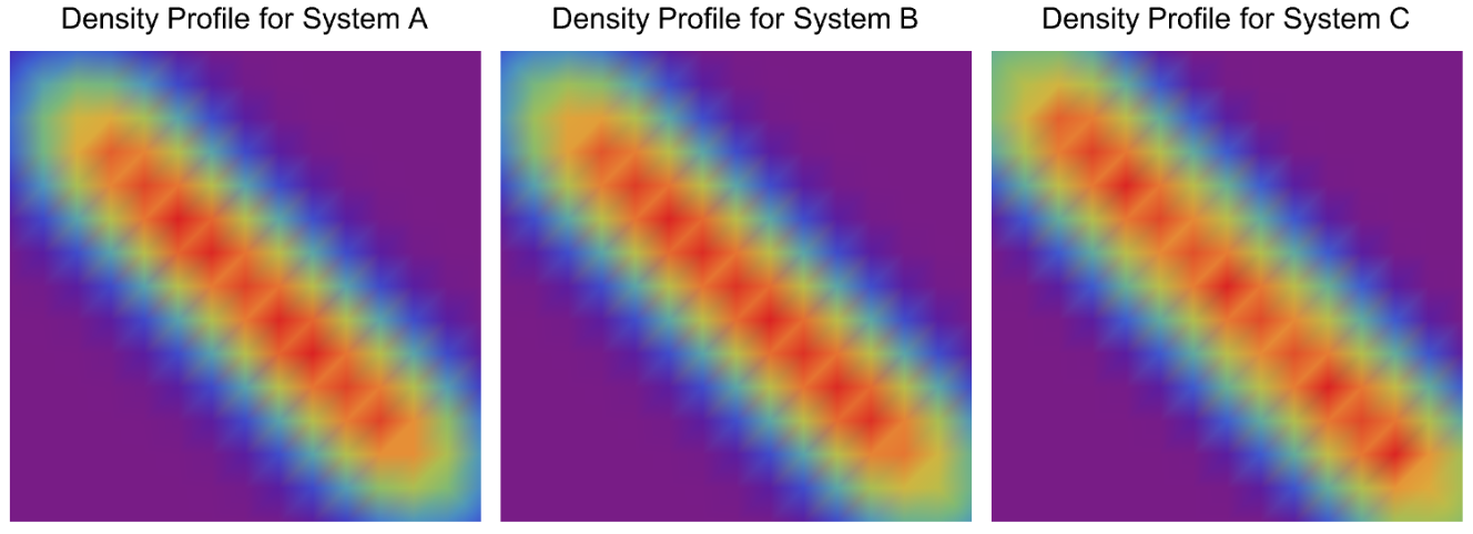
We begin the study by setting up a classical simulation: a particle cluster was shoot from the left-upper corner to the right-lower corner and scattered into random gas dynamics [Wolfram, 2022]. The hypothesis is the original system contains particles as a cluster, nominated as system C. This system can be coarse-grained to a cluster with particles ( particle), nominated as system B. System C can also be coarse-grained to a cluster with particles ( particle), nominated as system A. We can then simulate the dynamics of the three systems and observe their corresponding macroscale dynamics as the density profiles.
3030
66
251
33
1001
In[]:=
viz1=ResourceFunction["HardSphereSimulation"][<|"Positions"->Catenate@Table[{-15+2.5 i,15-2.5 j},{i,3},{j,3}],"Velocities"->Table[.5 {1,-1},9],"BoxSize"->30,"StepSize"->0.5,"ParticleRadius"->1,"Steps"->10,"BoundaryCondition"->"Reflecting","Output"->"Visualize"|>];viz2=ResourceFunction["HardSphereSimulation"][<|"Positions"->Catenate@Table[{-14.375+1.25 i,14.375-1.25 j},{i,6},{j,6}],"Velocities"->Table[.5 {1,-1},36],"BoxSize"->30,"StepSize"->0.5,"ParticleRadius"->0.5,"Steps"->10,"BoundaryCondition"->"Reflecting","Output"->"Visualize"|>];viz3=ResourceFunction["HardSphereSimulation"][<|"Positions"->Catenate@Table[{-14+.25 i,14-.25 j},{i,30},{j,30}],"Velocities"->Table[.5 {1,-1},900],"BoxSize"->30,"StepSize"->0.5,"ParticleRadius"->0.1,"Steps"->10,"BoundaryCondition"->"Reflecting","Output"->"Visualize"|>];Row[{viz1,viz2,viz3}]
Out[]=

In[]:=
colls9par=ResourceFunction["HardSphereSimulation"][<|"Positions"->Catenate@Table[{-15+2.5 i,15-2.5 j},{i,3},{j,3}],"Velocities"->Table[.5 {1,-1},9],"BoxSize"->30,"StepSize"->0.5,"ParticleRadius"->1,"Steps"->10000,"BoundaryCondition"->"Reflecting","ParticleMass"->1,"Output"->"PositionsByParticle"|>];colls36par=ResourceFunction["HardSphereSimulation"][<|"Positions"->Catenate@Table[{-14.375+1.25 i,14.375-1.25 j},{i,6},{j,6}],"Velocities"->Table[.5 {1,-1},36],"BoxSize"->30,"StepSize"->0.5,"ParticleRadius"->0.5,"Steps"->10000,"BoundaryCondition"->"Reflecting","ParticleMass"->1/9,"Output"->"PositionsByParticle"|>];colls900par=ResourceFunction["HardSphereSimulation"][<|"Positions"->Catenate@Table[{-14+.25 i,14-.25 j},{i,30},{j,30}],"Velocities"->Table[.5 {1,-1},900],"BoxSize"->30,"StepSize"->0.5,"ParticleRadius"->0.1,"Steps"->10000,"BoundaryCondition"->"Reflecting","ParticleMass"->1/100,"Output"->"PositionsByParticle"|>];
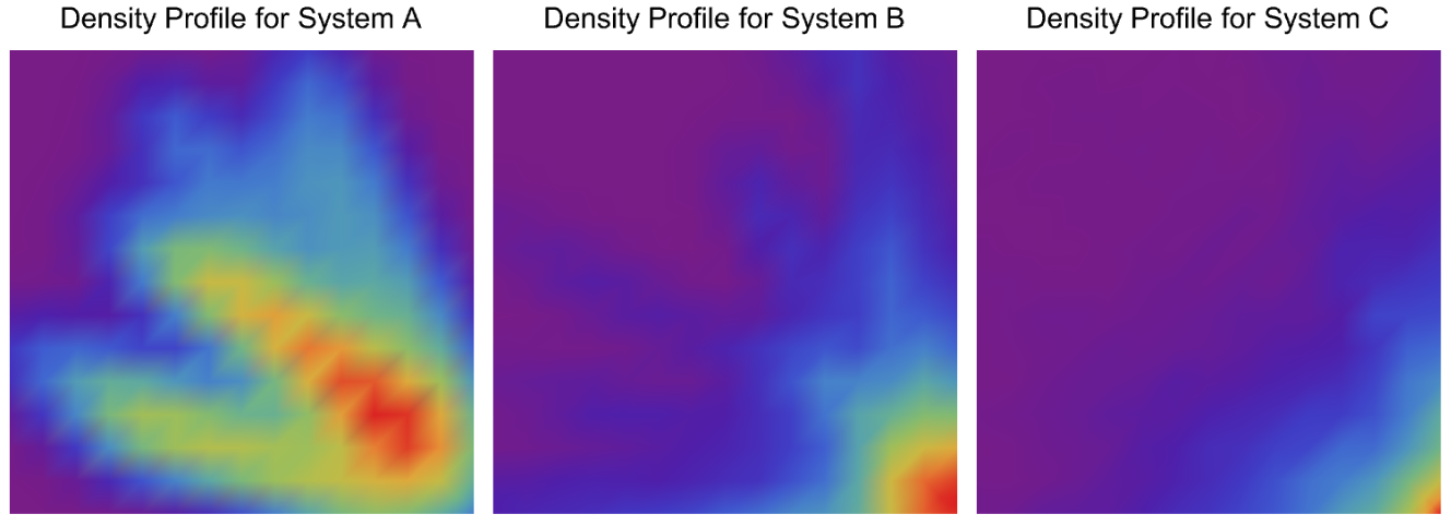
This whole process can be decomposed into three regimes: (1) the process from the left corner to the right corner, considered as the pseudo-flow dynamics; (2) the moment when the collision happens, considered as the collision dynamics; (3) random motion of the particles within the box, considered as random particle dynamics. The three macro density profiles of the three regimes are shown as flows.
Regime 1 : Particle Cluster Pseudo - Flow Dynamics
In[]:=
overall9parregime1=Flatten[colls9par[[All,1;;90,All]],1];overall36parregime1=Flatten[colls36par[[All,1;;90,All]],1];overall900parregime1=Flatten[colls900par[[All,1;;90,All]],1];Row[{over9parsmoothregime1=SmoothDensityHistogram[overall9parregime1,PlotRange->{-15,15},Frame->None,ImagePadding->0,ColorFunction->"Rainbow",PlotLabel->Style["Density Profile for System A",Black, 15],ImageSize->250],over36parsmoothregime1=SmoothDensityHistogram[overall36parregime1,PlotRange->{-15,15},Frame->None,ImagePadding->0,ColorFunction->"Rainbow",PlotLabel->Style["Density Profile for System B",Black, 15],ImageSize->250],over900parsmoothregime1=SmoothDensityHistogram[overall900parregime1,PlotRange->{-15,15},Frame->None,ImagePadding->0,ColorFunction->"Rainbow",PlotLabel->Style["Density Profile for System C",Black, 15],ImageSize->250]}]
Out[]=
Regime 2 : Particle Cluster Collision Dynamics
In[]:=
overall9parregime2=Flatten[colls9par[[All,90;;150,All]],1];overall36parregime2=Flatten[colls36par[[All,90;;150,All]],1];overall900parregime2=Flatten[colls900par[[All,90;;150,All]],1];Row[{over9parsmoothregime2=SmoothDensityHistogram[overall9parregime2,PlotRange->{-15,15},Frame->None,ImagePadding->0,ColorFunction->"Rainbow",PlotLabel->Style["Density Profile for System A",Black, 15],ImageSize->250],over36parsmoothregime2=SmoothDensityHistogram[overall36parregime2,PlotRange->{-15,15},Frame->None,ImagePadding->0,ColorFunction->"Rainbow",PlotLabel->Style["Density Profile for System B",Black, 15],ImageSize->250],over900parsmoothregime2=SmoothDensityHistogram[overall900parregime2,PlotRange->{-15,15},Frame->None,ImagePadding->0,ColorFunction->"Rainbow",PlotLabel->Style["Density Profile for System C",Black, 15],ImageSize->250]}]
Out[]=
Regime 3 : Discretize Random Particle Dynamics
overall9parregime3 = Flatten[colls9par[[All,150 ;; 9000,All]], 1]; overall36parregime3 = Flatten[colls36par[[All,150 ;; 9000,All]], 1]; overall900parregime3 = Flatten[colls900par[[All,150 ;; 9000,All]], 1]; figpar9rgm3 = SmoothDensityHistogram[overall9parregime3, PlotRange -> All, Frame -> None, ImagePadding -> 0]; figpar9rgm3 = Image[figpar9rgm3, ImageSize -> 150, ImageResolution -> 72]; figpar9rgm3 = ImageData[figpar9rgm3]; figpar9rgm3 = Transpose[figpar9rgm3, {2, 3, 1}]; figpar9rgm3 = figpar9rgm3[[1 ;; All, 11 ;; 140, 11 ;; 140]];figpar36rgm3 = SmoothDensityHistogram[overall36parregime3, PlotRange -> All, Frame -> None, ImagePadding -> 0]; figpar36rgm3 = Image[figpar36rgm3, ImageSize -> 150, ImageResolution -> 72]; figpar36rgm3 = ImageData[figpar36rgm3]; figpar36rgm3 = Transpose[figpar36rgm3, {2, 3, 1}]; figpar36rgm3 = figpar36rgm3[[1 ;; All, 11 ;; 140, 11 ;; 140]];figpar900rgm3 = SmoothDensityHistogram[overall900parregime3, PlotRange -> All, Frame -> None, ImagePadding -> 0]; figpar900rgm3 = Image[figpar900rgm3, ImageSize -> 150, ImageResolution -> 72]; figpar900rgm3 = ImageData[figpar900rgm3]; figpar900rgm3 = Transpose[figpar900rgm3, {2, 3, 1}]; figpar900rgm3 = figpar900rgm3[[1 ;; All, 11 ;; 140, 11 ;; 140]];
The visualizations above show that for both three regimes, similar density profiles for different coarse-grained systems. However, from the observations, one can only argue that based on rough observations it is difficult to extract the small differences between other systems, but one cannot quantitatively argue that the different coarse-grained systems have similar dynamics under specific criteria. To strengthen the argument, we first need to detect the exact differences between the details of other systems. We decomposed the whole particle motion into snapshots to capture the local dynamics of the motion directly and visualize it as follows.
Local Dynamics
Local Dynamics
System A
System A contains 9 particles, and the density profile is extracted based on the spatial distribution of the particle at different time steps.
System B
System B contains 36 particles, and the density profile is extracted based on the spatial distribution of the particle at different time steps.
System C
System C contains 900 particles, and the density profile is extracted based on the spatial distribution of the particle at different time steps.
In this section, we directly visualize the physical intuition under particle-based coarse-graining: the macroscale observation, i.e., the density profile, is observed to be similar. However, from both mathematical and physical perspectives, this is not a strong argument as there is no exact quantitative or symbolic analysis directing this evidence. Following the idea, we first show the differences in the local dynamics and are to show how to characterize these different coarse-grained systems using graph models in the following section.
Characterization of Spatial Coarse-Grain
Characterization of Spatial Coarse-Grain
The Spatial Coarse-Grain Approach for Equilibrium Process
The Spatial Coarse-Grain Approach for Equilibrium Process
Following the previous sections, one can deduce that the three regimes of the illustrative example contain two nonequilibrium (flow and collision) and one equilibrium (random motion) process. As we did not modify the forcefield (hard sphere gas models), the larger particle does not preserve the hierarchical dynamics of the smaller particles, i.e., a larger particle cannot represent multiple smaller particles after a collision happens when the motion of smaller particles are randomized at a smaller time scale. This indicates that using this kind of coarse-graining to study the nonequilibrium process is not physically rigorous.
However, equilibrium processes, physically different coarse-grained systems confined in the box running for a long time until the overall thermodynamical properties of the systems reach the same, possess clear criteria to study and measure, e.g., Maxwell-Boltzmann function. One may also check the local dynamics of such systems, e.g., the collective behavior of all the particles in the box in the short time regime.
Here, we investigate the equilibrium process. Assuming we have two systems containing 9 and 36 particles respectively. We want to look at both the hypergraphs and causal graphs of the two systems for the examination of the coarse-graining. We first run the two systems until thermodynamic equilibrium.
The left visualization corresponds to the case of the 9-particle system and the right corresponds to the case of the 36-particle system.
Thermodynamics
Thermodynamics
To check the thermodynamical equilibrium of the two systems, one can check the distribution of speeds w.r.t. temperature and fit with the Maxwell-Boltzmann function, shown as follows.
For a detailed analysis of these equilibrium systems using hypergraphs and causal graphs, please check Supplementary Section I and Supplementary Section II in the Appendix.
Spatial and Temporal Coarse-Graining
Spatial and Temporal Coarse-Graining
There are two ways to do coarse-grain to reduce the order of the system for reduced computational costs, spatial and temporal. For spatial, we take the common approach used in the discrete element communities, which assumes by enlarging the particle size and decreasing the particle numbers in ratio, the macroscopic behavior of the system should roughly be the same. We compare different systems of the same box running with the same time steps but with different particle numbers and radii. We examine this assumption by testing the linear relation between the collision rate and the square root of the temperature. For the temporal coarse-grain approach, we directly operate on the causal graph by uniformly subtracting the “extra” node (representing the collision events) from the overall causal graph. By resampling the causal and assign with new labels to represent the density of the new nodes, the temporal coarse-grained causal graph is able to preserve the collision rates.
The two approaches are introduced and examined in different cases with different particle sizes and numbers. Their corresponding assumptions, verifications, and limitations are then briefly elaborated on and discussed. Most importantly, we indicate under which scenario these coarse-grain approaches then tend to fail, i.e., preserve the physics of the original system.
The two approaches are introduced and examined in different cases with different particle sizes and numbers. Their corresponding assumptions, verifications, and limitations are then briefly elaborated on and discussed. Most importantly, we indicate under which scenario these coarse-grain approaches then tend to fail, i.e., preserve the physics of the original system.
Examine the Physics from the Causal Graph for Spatial Coarse-Graining
Examine the Physics from the Causal Graph for Spatial Coarse-Graining
A very interesting phenomenon is observed: those different “coarse-grained” systems (we can think of the original system as a system with a coarse-grain degree of zero) all obey the ideal gas law with very similar fitting parameters (slope)! This indicates that the different coarse-grained systems can be interpreted as a surrogate for each other pertaining to the thermodynamics properties considering collision rate and temperature according to the ideal gas law. However, one may also argue that the short-time collective behavior of those different coarse-grained systems is still different even though their overall relationships are similar. Hence, we generate the following figures to show the velocity correlation (decay of particle velocities correlation w.r.t. time) and kinetic energy evolution w.r.t. time.
Admittedly, it is intuitive that one may expect a large particle may have a slower velocity correlation than the smaller particles (If not in a coarse-grained system this may be true, e.g., with similar particle numbers). However, the two left figures above show that all five different coarse-grained systems possess similar velocity correlation properties, indicating the collective particle behavior in the short-time regime is similar. Also, the total kinetic energy fluctuation w.r.t. time shows that the collective kinetic energies are preserved well for different coarse-grained systems tested, with no obvious differences detected.
Along with the collision rates, this shall be a shred of direct quantitative evidence showing that the spatial coarse-graining preserves physical properties for thermodynamically equilibrium systems.
Along with the collision rates, this shall be a shred of direct quantitative evidence showing that the spatial coarse-graining preserves physical properties for thermodynamically equilibrium systems.
Examine the Physics from the Causal Graph for Temporal Coarse-Graining
Examine the Physics from the Causal Graph for Temporal Coarse-Graining
Now, we directly operate on the causal by cutting out edges for coarse-graining the causal graph. The way we propose to coarse-grain the causal graph is to uniformly sample the node that represent the collision events and cut off by assigned quantities. For example, if one has a list representing the node: {1,2,3,4,5,6,7,8,9,10}, assume this list stand for a causal graph representing a series of events with the ordered label, we can get the coarse-grained causal graph by simply extract by arithmetic order. Say one wants to get the coarse-grained graph preserving half the nodes, i.e., by the order of 2, the new graph writes: {1,3,5,7,9}. Similarly, if one wants to obtain a coarse-grained graph by the order of 3, one obtain a new graph {1,4,7,10}.
Now, the problem here would be if the node numbers in the graph are small, then by doing this kind of “coarse-graining” one cannot guarantee the new graph possesses exacting the information memory one hopes to keep. From our previous example by sampling differently the “order-3” coarse-grained graph contains either 3 or 4 nodes. Putting this in the general case of simulating hard sphere models one concludes that the collision events one stores in the new graph may contain unavoidable errors. But with the increase of causal graph size this error with become relatively smaller until it eventually yields to zero.
Here, we begin with a toy example to illustrate what this kind of coarse-graining looks like, and then we implement this coarse-grain technique to particle systems or larger scales. We will briefly elaborate on the pros and cons of such an approach and how this approach may further inspire a graph-based approach to better understand physics.
Here, we begin with a toy example to illustrate what this kind of coarse-graining looks like, and then we implement this coarse-grain technique to particle systems or larger scales. We will briefly elaborate on the pros and cons of such an approach and how this approach may further inspire a graph-based approach to better understand physics.
A Toy Example
A Toy Example
We begin with the System A we just used and run for only 50 steps as it only contains a few collision events so we could better illustrate how the causal graph is coarse-grained.
The causal graph shows the collisions hidden beneath the toy example. The label on each node stands for the labels of the two particles involved in the collision and the third element is the corresponding collision time. One can observe that on this causal graph, each node contains the label of different particles and the corresponding time at each collision. Just from the causal graph, one can directly compute the collision rate by counting the total number of nodes first and dividing by the simulation time. In order to coarse-grain this causal graph, we first assign a value of “1” at the end of each node element:
We then do the coarse-grained sampling procedure on this causal graph, by the order of 2. We first extract the nodes in arithmetic order using the method we just mentioned and reassign the tale value as 2:
We can then check the total number of collisions by summarizing the tale values:
The collision numbers deviate from the ground truth by 1, although sometimes they could be the same (as explained previously). We can then compute the collision rates of the two different causal graphs (that are expected to be similar since the total time is the same) to show how the thermodynamics quantities are preserved on the coarse-grained causal graph(s).
We start the computation by obtaining the final time of the whole collision process:
We start the computation by obtaining the final time of the whole collision process:
The collision rate for both the two systems are then:
The collision rate results deviate a little because the two final times of the two systems are different caused by our sampling. However, these collision rates are expected to be the same under larger systems since the deviation of the time would not matter to the total collisions as much compared to the toy case here with total collisions of only 80. To better understand what we did on the toy system, we visualize the graph from the new collisions compared with the old one.
Practice on Coarse-Graining on Causal Graph for Large Scale Systems
Practice on Coarse-Graining on Causal Graph for Large Scale Systems
Now we will use a thermodynamical equilibrium system (large system with long time steps) to conduct the causal graph coarse-grain based on our general formulation shown above. We begin with a system of 100 particles running for 5000 time steps and do coarse-graining on its corresponding causal graph.
We check the systems reach equilibrium by testing its corresponding Maxwell-Boltzmann fit:
It can be deduced that this is an equilibrium system. We can hence operate the coarse-graining procedure we did on the toy example to this system. The key is due to the large size of this system, we may not be able to directly visualize the causal graph from the simulation. But we can examine the statistics of the causal graph, which is both mathematical and physically more interesting to understand this “sample and filter” approach.
We then do the coarse grain on our causal graph with five different degrees, just as what we did for the spatial coarse-grain:
Concluding remarks
Concluding remarks
Keywords
Keywords
◼
Hard Sphere Simulations
◼
Statistical Mechanics
◼
Coarse Graining
◼
Multiscale Modeling
◼
Causal Graph
◼
Thermodynamics
◼
Computational Physics
◼
Computational Irreducibility
◼
Model Reduction
Acknowledgement
Acknowledgement
I would like to thank my mentors Sotiris Michos, Nik Murzin, and James Boyd for constantly providing me with technical guidance, feedback, support, and advice on this project. I would also like to thank Matt Kafker, the developer of hard sphere simulation models in Wolfram language, for his selfless contribution to this project, especially for his key ideas and insight and for taking the time to provide me with tutorials and guidance. I would also like to Stephen Wolfram, for assigning me this project, providing his unique insights on multiscale modeling, and for the amazing discussions during the Winter School. I would also like to thank Zach Shelton, for providing computational and technical support in Wolfram technologies through the Wolfram Student Ambassador Program. The amazing research talks and discussions held during the Winter School lead me to the exciting projects and works conducted at Wolfram Research.
References
References
◼
[Thoennessen, 1995] Michael Thoennessen. Gas Laws and Kinetic Theory. URL: https://people.nscl.msu.edu/~thoennes/personal/phy231/p231_notes6.pdf.
◼
[Wolfram, 2022] Stephen Wolfram. On the Concept of Motion. URL: https://writings.stephenwolfram.com/2022/03/on-the-concept-of-motion/
◼
[Kafker, 2020] Matt Kafker. [WSS20] Exploring Networks in Hard Sphere Models. URL: https://community.wolfram.com/groups/-/m/t/2028871
◼
[Widartiningsih et al., 2020] Putri Mustika Widartiningsih et al. Coarse graining DEM simulations of a powder die-filling system. Powder Technology. URL: https://doi.org/10.1016/j.powtec.2020.05.063
◼
[Kanjilal & Schneiderbauer, 2021] Suranita Kanjilal and Simon Schneiderbauer. A revised coarse-graining approach for simulation of highly poly-disperse granular flows. Powder Technology. URL: https://doi.org/10.1016/j.powtec.2021.02.015
◼
[Lu et al., 2016] Liqiang Lu et al. Coarse-Grained-Particle Method for Simulation of Liquid–Solids Reacting Flows. Ind. Eng. Chem. Res. URL: https://doi.org/10.1021/acs.iecr.6b02688
◼
[Wolfram, 2002] Stephen Wolfram. A New Kind of Science. URL: https://www.wolframscience.com/nks/
Appendix
Appendix
Supplementary Codes
Supplementary Codes