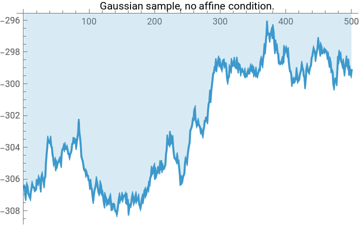
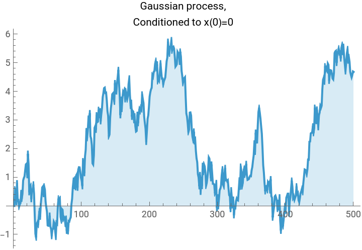
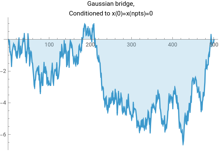
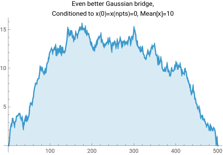
TLDR is that if we have a Gaussian , and we want to condition on the linear system of conditions , then we simply project: This gives us a fun way to look at a few different Gaussian processes using the same code:
x∼N(0,Σ)
Lx=b
x↦x+Σ(b-Lx).
T
L
-1
(LΣ)
T
L
In[]:=
(*Randomsampleofa1Dscalarfieldwithenergyfunction(akax.Hessian.xakax.precisionmatrix.x)E=\sum_iK(-x_i(x_{i+1}+x_{i-1}-2x_i)+m^2x_i^2),subjecttolinearconstraintsl.x==b.Freeboundaryconditionsareassumed,soweneedm>0fortheproblemtobewell-defined.*)gaussianField1D[npts_,m_,k_,l_:{},b_:{}]:=Module[{cov,hessian,sample,dist},(*Constructthehessiandesired.Therulesspecifiedfirsttakeprecedence,thenwespecifythediagonalbands.*)hessian=SparseArray[{{1,1}->m^2+k,{npts,npts}->m^2+k,Band[{1,1}]->m^2+2k,Band[{1,2}]->-k,Band[{2,1}]->-k},{npts,npts}];cov=Inverse[hessian];sample=RandomVariate[MultinormalDistribution[cov]];Which[(*case1,noconditions*)Length[l]==0,sample,(*case2,oneaffinecondition*)Dimensions[l]=={npts},sample+cov.l/(l.cov.l)(b-l.sample),(*case3,multipleaffineconditions*)Length[Dimensions[l]]==2,sample+cov.Transpose[l].Inverse[l.cov.Transpose[l]].(b-l.sample)]];npts=500;myplot[vector_,label_]:=ListLinePlot[vector,PlotLabel->Style[label,Black],ImageSize->Medium,Filling->Axis];plot1=myplot[gaussianField1D[npts,0.0001,10],"Gaussian sample, no affine condition."];plot2=myplot[gaussianField1D[npts,0.0001,10,Table[If[i==1,1,0],{i,1,npts}],0],"Gaussian process,\nConditioned to x(0)=0"];plot3=myplot[gaussianField1D[npts,0.0001,10,{Table[If[i==1,1,0],{i,1,npts}],Table[If[i==npts,1,0],{i,1,npts}]},{0,0}],"Gaussian bridge,\nConditioned to x(0)=x(npts)=0"];plot4=myplot[gaussianField1D[npts,0.0001,10,{Table[If[i==1,1,0],{i,1,npts}],Table[If[i==npts,1,0],{i,1,npts}],Table[1/npts,{i,1,npts}]},{0,0,10}],"Even better Gaussian bridge,\nConditioned to x(0)=x(npts)=0, Mean[x]=10"];Grid[{{plot1,plot2},{plot3,plot4}},Frame->All]
Out[]=
In[]:=
dim=500;nsamples=10^6;(*findafunpositivedefinitesymmetricmatrixsigma*)sigma=RandomReal[{0,1},{dim,dim}];sigma=sigma+Transpose[sigma];sigma=sigma-IdentityMatrix[dim](Min[Eigenvalues[sigma]]-1);testAccuracy[sample_]:=Norm[sample.Transpose[sample]/nsamples-sigma];(*Exactdiagonalization*)normalize[v_]:=v/Sqrt[v.v];AbsoluteTiming[sampleDiagonal=Module[{d,pt,p},{d,pt}=Eigensystem[sigma];p=normalize/@Transpose[pt];p.(Sqrt[d]RandomVariate[NormalDistribution[],{dim,nsamples}])];testAccuracy[sampleDiagonal]](*Choleskydecomposition*)AbsoluteTiming[sampleCholesky=Module[{ll},ll=CholeskyDecomposition[sigma];Transpose[ll].RandomVariate[NormalDistribution[],{dim,nsamples}]];testAccuracy[sampleCholesky]](*Multinormal*)AbsoluteTiming[sampleMultinormal=Transpose@RandomVariate[MultinormalDistribution[sigma],nsamples];testAccuracy[sampleMultinormal]]
Out[]=
{9.03227,2.22439}
Out[]=
{8.438,2.1805}
Out[]=
{8.90825,2.44853}
In[]:=
hessian=Inverse[sigma];(*numericalinstabilitiesintheinversemakesurethehessianissymmetric*)hessian=(hessian+Transpose[hessian])/2;(*Choleskydecomposition*)AbsoluteTiming[sampleHessian=Module[{solver,ll},ll=CholeskyDecomposition[hessian];solver=LinearSolve[ll];solver[RandomVariate[NormalDistribution[],{dim,nsamples}]]];testAccuracy[sampleHessian]]
Out[]=
{9.30303,2.44486}