ABSTRACT (original article): Cross-sections of cell shapes in a tissue monolayer typically resemble a tiling of convex polygons. Yet, examples exist where the polygons are not convex with curved cell–cell interfaces, as seen in the adaxial epidermis. To date, two-dimensional vertex models predicting the structure and mechanics of cell monolayers have been mostly limited to convex polygons. To overcome this limitation, we introduce a framework to study curvy cell–cell interfaces at the subcellular scale within vertex models by using a parametrized curve between vertices that is expanded in a Fourier series and whose coefficients represent additional degrees of freedom. This extension to non-convex polygons allows for cells with the same shape index, or dimensionless perimeter, to be, for example, either elongated or globular with lobes. In the presence of applied, anisotropic stresses, we find that local, subcellular curvature or buckling can be energetically more favourable than larger scale deformations involving groups of cells. Inspired by recent experiments, we also find that local, subcellular curvature at cell–cell interfaces emerges in a group of cells in response to the swelling of additional cells surrounding the group. Our framework, therefore, can account for a wider array of multicellular responses to constraints in the tissue environment. CITATION (original article): Kim Kyungeun, Schwarz J. M. and Ben Amar Martine (2024), A two-dimensional vertex model for curvy cell–cell interfaces at the subcellular scale. J. R. Soc. Interface. 21:20240193. http://doi.org/10.1098/rsif.2024.0193
Preprint arXiv: https://arxiv.org/abs/2403.14417
Preprint arXiv: https://arxiv.org/abs/2403.14417
Introduction
Introduction
Vertex models have traditionally represented tissue cells as space-filling polyhedrons with straight edges to understand cellular interactions and tissue behavior. However, many plant and animal tissues exhibit cells with curved edges, likely due to actomyosin cortex reorganization. This curved geometry allows cells to increase their surface area while maintaining volume and can influence tissue properties like fluidity. Recent observations of curved cell-cell interfaces in various biological contexts demonstrate the biological significance of these curved geometries. To better understand these systems, a modified two-dimensional vertex model has been developed that incorporates curved cell-cell interfaces using parameterized curves with Fourier coefficients, enabling exploration of conditions favoring straight versus curved edges and providing insights into how subcellular shape regulation affects tissue-scale phenomena.
In[]:=
SetDirectory[NotebookDirectory[]];
In this notebook, we will show how we simulate curved-edged cell using energy minimization. Throughout this note, we have used NMinimize with Nelder-Mead methods.
We recommend using provided results instead of independent execution due to long computation time.
We recommend using provided results instead of independent execution due to long computation time.
Cell energy functions: E=(A_i-A_0)^2+(P_i-P_0)^2 or E=(p_i-p_0)^2 where:
- A_i: current cell area
- A_0: target area
- P_i: current cell perimeter
- P_0: target perimeter
- p_i: shape index of current cell
- p_0: target shape index
- A_i: current cell area
- A_0: target area
- P_i: current cell perimeter
- P_0: target perimeter
- p_i: shape index of current cell
- p_0: target shape index
Definitions and functions for hexagon shape analysis
Definitions and functions for hexagon shape analysis
Properties of the curved-edged model
Properties of the curved-edged model
A. Transition from convex to non-convex for a single cell
A. Transition from convex to non-convex for a single cell
Example (related to Fig. 5a): We minimize (p_i - p_0)^2, where p_0 is the target shape index set to that of a circle (~3.5). This comparison demonstrates the advantages of our curved-edge cell model, as traditional straight-edge models (based on hexagons) cannot achieve shape indices below that of a regular hexagon (~3.7).
Define the basic structure for a single hexagon . Note : This implementation differs from the paper but calculates the shape index for a hexagon instead of wedge using the similar equation.
SingleHex=GraphicsComplex[{{0.8660254038`,0.5`},{0.`,1.`},{-0.8660254038`,0.5`},{-0.8660254038`,-0.5`},{0.`,-1.`},{0.8660254038`,-0.5`}},{Polygon[{1,2,3,4,5,6}]}];
Polygon vertices list - Define the vertex indices for the polygon Format : {{polygon1_vertices}, {polygon2_vertices}, ...}
spmat={{1,2,3,4,5,6}};
Edge connectivity matrix - Defines how vertices are connected Each pair represents an edge between two vertices
scm={{1,2},{2,3},{3,4},{4,5},{5,6},{6,1}};
Mapping between polygon list and edge list Associates edges with their corresponding polygons
scxsort={{1,2,3,4,5,6}};
Convert 2 D vertex array to 1 D array for processing
svpt=Flatten[SingleHex[[1]],1];
Goal: Analyze how a hexagon can transform into a circle-Circle shape index≈3.55
Optimization function: (Perimeter/Sqrt[total area]-3.5)^2 -> (Shape Index-3.5)^2
where total area=polygon area + curved part area
Components in minimizer: fl0dapprox:Perimeter-Farea:Polygon area-fsdapproxnosq:Area of curved parts
Optimization function: (Perimeter/Sqrt[total area]-3.5)^2 -> (Shape Index-3.5)^2
where total area=polygon area + curved part area
Components in minimizer: fl0dapprox:Perimeter-Farea:Polygon area-fsdapproxnosq:Area of curved parts
Fixed coordinate indices
sbd={1,2,3,4,5,6};
Configuration parameters
vnum=12;(*Numberofcoordinatevectors*)cnum=24;(*Numberofedgecoefficients:4harmonics×6edges*)
Optimization setup
(*Initializecoefficientarraywithoptimizationvariables*)sc=Array[x,vnum+cnum];(*Optimizationobjectiveexplained:1.Regularizationterm:Controlscoefficientmagnitudes(0.1*Σ(coeff-0.05)²)2.Shapeindexterm:Minimizesdifferencefromcircle1.5*perimeter√area-3.5²Note:3.5istargetvalue,whiletruecirclehas3.553.Boundaryconstraints:Maintainsgeometricvalidity(Fresbdterm)*)ssol=sc/.Last[With[{sc=Array[x,vnum+cnum]},NMinimize[0.1*Sum[(sc[[i]]-0.05)^2,{i,vnum+1,vnum+cnum}]+1.5*((fl0dapprox[sc[[1;;vnum]],spmat,sc[[vnum+1;;vnum+cnum]],scxsort,1]/Sqrt[Farea[sc[[1;;vnum]],spmat,1]+fsdapproxnosq[sc[[1;;vnum]],spmat,sc[[vnum+1;;vnum+cnum]],scxsort,1]])-3.5)^2+Fresbd[sc,svpt,sbd,1000],sc,Method->"NelderMead"]]]
Out[]=
{0.852469,0.492173,-4.24219×,0.984347,-0.852469,0.492173,-0.852469,-0.492173,3.21643×,-0.984347,0.852469,-0.492173,0.109788,0.00588769,0.00824007,0.00171713,0.109788,0.00588768,0.00824007,0.00171713,0.109788,0.00588768,0.00824007,0.00171713,0.109788,0.00588768,0.00824006,0.00171713,0.109788,0.00588768,0.00824006,0.00171713,0.109788,0.00588768,0.00824006,0.00171713}
-9
10
-9
10
In[]:=
cxsol=Table[{ssol[[2i-1]],ssol[[2i]]},{i,1,12}];cx=Table[ssol[[i]],{i,13,36}];
In[]:=
Show[Graphics[{EdgeForm[Thick],Dashed,Gray,Line[Table[{cxsol[[scm[[i,1]]]],cxsol[[scm[[i,2]]]]},{i,1,6}]]}],ParametricPlot[{Table[{fs[{ssol[[2*scm[[i,1]]-1]],ssol[[2*scm[[i,1]]]],ssol[[2*scm[[i,2]]-1]],ssol[[2*scm[[i,2]]]]},cx[[4i-3]],cx[[4i-2]],cx[[4i-1]],cx[[4i]],t],gs[{ssol[[2*scm[[i,1]]-1]],ssol[[2*scm[[i,1]]]],ssol[[2*scm[[i,2]]-1]],ssol[[2*scm[[i,2]]]]},cx[[4i-3]],cx[[4i-2]],cx[[4i-1]],cx[[4i]],t]},{i,1,6}]},{t,0,1},PlotStyle->{Thickness[0.005],Blue}],ImageSize->Medium]
Out[]=
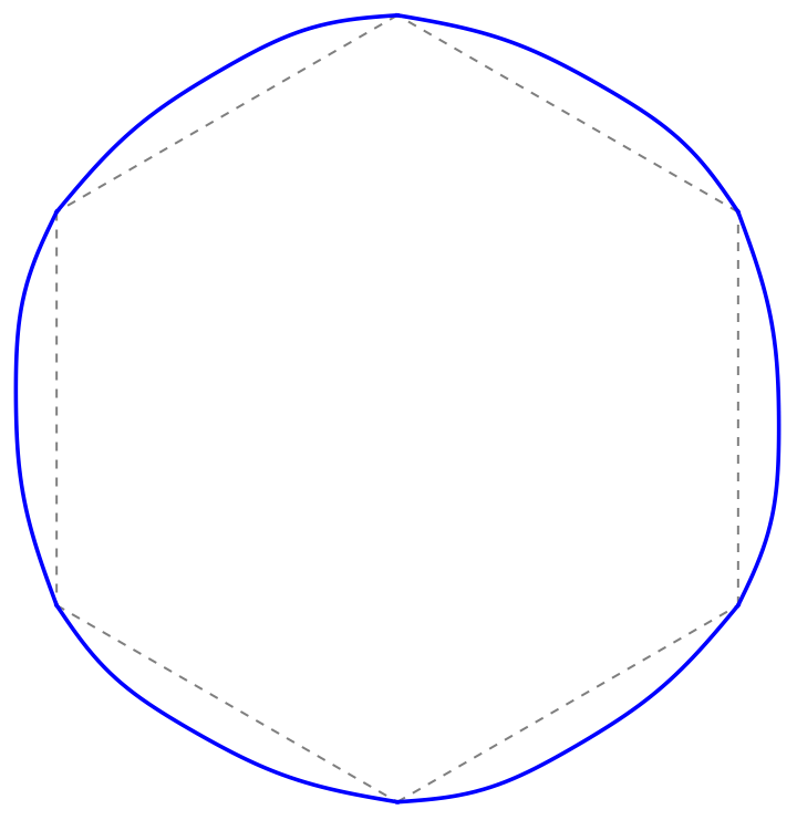
Note: The shape index approaches but will not exactly reach 3.5 due to the physical limit of shape index minimum (~3.55). For target > 3.55, there could be errors from curved-edged part calculations and numerical optimization constraints. The initial sinusoidal coefficients (0.05) may also not be optimal for reaching the target shape index.
Calculate and verify the final shape index
fl0dapprox[ssol[[1;;vnum]],spmat,ssol[[vnum+1;;vnum+cnum]],scxsort,1]/Sqrt[Farea[ssol[[1;;vnum]],spmat,1]+fsdapproxnosq[ssol[[1;;vnum]],spmat,ssol[[vnum+1;;vnum+cnum]],scxsort,1]]
Out[]=
3.54929
A2. Simulation conditions for compression-induced curved edges
A2. Simulation conditions for compression-induced curved edges
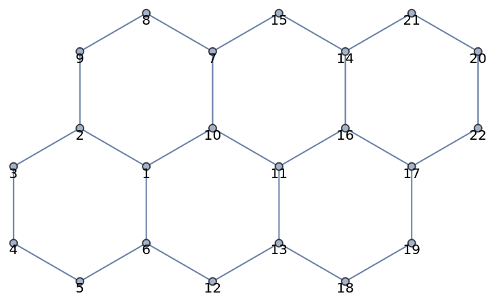
Example (shown in Figure A1 (a) in the appendix): The system consists of six ordered hexagonal cells stacked together. We minimize the energy function using both area and perimeter constraints, expressed as Minimize[(A_i-A_0)^2+(P_i-P_0)^2], where A_i and P_i are the current area and perimeter, while A_0 and P_0 are the target area and perimeter respectively.
Analysis configuration for 6 connected hexagons arrangement
Polygon vertex list - defines vertex indices for each hexagon
Polygon vertex list - defines vertex indices for each hexagon
Hex=GraphicsComplex[{{0.8660254038`,0.5`},{0.`,1.`},{-0.8660254038`,0.5`},{-0.8660254038`,-0.5`},{0.`,-1.`},{0.8660254038`,-0.5`},{1.7320508076`,2.`},{0.8660254038`,2.5`},{0.`,2.`},{1.7320508076`,1.`},{2.5980762114`,0.5`},{1.7320508076`,-1.`},{2.5980762114`,-0.5`},{3.4641016151`,2.`},{2.5980762114`,2.5`},{3.4641016151`,1.`},{4.3301270189`,0.5`},{3.4641016151`,-1.`},{4.3301270189`,-0.5`},{5.1961524227`,2.`},{4.3301270189`,2.5`},{5.1961524227`,1.`}},{Polygon[{1,2,3,4,5,6}],Polygon[{7,8,9,2,1,10}],Polygon[{11,10,1,6,12,13}],Polygon[{14,15,7,10,11,16}],Polygon[{17,16,11,13,18,19}],Polygon[{20,21,14,16,17,22}]}];
Polygon vertices list - Define the vertex indices for the polygon Format : {{polygon1_vertices}, {polygon2_vertices}, ...}
pmat={{1,2,3,4,5,6},{7,8,9,2,1,10},{11,10,1,6,12,13},{14,15,7,10,11,16},{17,16,11,13,18,19},{20,21,14,16,17,22}};
Edge connectivity matrix - Defines how vertices are connected Each pair represents an edge between two vertices
cm={{1,2},{1,6},{1,10},{2,3},{2,9},{3,4},{4,5},{5,6},{6,12},{7,8},{7,10},{7,15},{8,9},{10,11},{11,13},{11,16},{12,13},{13,18},{14,15},{14,16},{14,21},{16,17},{17,19},{17,22},{18,19},{20,21},{20,22}};
Mapping between polygon list and edge list Associates edges with their corresponding polygons . Example : Edge (1, 2) is 1 st element in cm, edge (5, 6) is 8 th element
cxsort={{1,4,6,7,8,2},{10,13,5,1,3,11},{14,3,2,9,17,15},{19,12,11,14,16,20},{22,16,15,18,25,23},{26,21,20,22,24,27}};
Graph representation of 6 connected hexagons Vertex numbering maps directly to positions in vertex list e . g ., vertex 1 in code corresponds to vertex 1 in visualization
gh=Graph[cm,VertexCoordinates->Hex[[1]]];GraphPlot[gh,VertexLabels->Placed[Automatic,Top]]
Out[]=
Fixed boundary vertices for stability These vertices remain stationary during optimization
bd={9,2,3,4,20,22,17,19};
Note: Fixed vertices are selected along the outer boundary to maintain the overall structure during shape deformation
Flatten 2 D vertex array into 1 D for processing Takes vertex coordinates from Hex[[1]] and converts to linear array
vpt=Flatten[Hex[[1]],1];
IMPORTANT: Performance Warning
- Code execution may cause Kernel reset depending on CPU capacity
- Save all work before running
- Recommended: Use provided results instead of independent execution
- Code execution may cause Kernel reset depending on CPU capacity
- Save all work before running
- Recommended: Use provided results instead of independent execution
Note: Extended computation time warning - Execution takes several minutes - Compare results with Soln_NminCE . txt for validation - Results may vary due to minimizer function strategy
Energy minimization configuration:
Objective function components:
1. Coefficient regularization : Target value 0.05
2. Perimeter constraint : Target length 6.2 (fl0dapprox)
3. Resistance function (Fressq) : Based on vertex positions (vpt) See paper for detailed explanation
4. Area conservation : Using Fareasq (squared polygon area)
Note: Parametric curve area (fsdapprox) not included in optimization due to negligible area changes from sinusoidal curves . Can be added if higher accuracy needed .
Use provided results
Visualization of optimization results - Gray dashed lines : Original polygon edges and vertices - Blue solid curves : Optimized curved edges - Computation time < 1 minute
Multicellular response to applied stresses
Multicellular response to applied stresses
B. Compression-induced curved edge
2. Disordered Cell Simulation
B. Compression-induced curved edge
2. Disordered Cell Simulation
2. Disordered Cell Simulation
Example (shown in Figure 12 (e,f)): The system consists of disordered hexagonal cells stacked together. We minimize the energy function using both area and perimeter constraints for boundary cells and interior cells, expressed as Minimize[(A_i^p-A_0)^2 (polygon) +(A_i^c)^2 (area under the curve to drive A_i^c=0)+(P_i^c-P_0)^2], where A_i^p and P_i^c are the current area and perimeter of curved-edged cells, while A_0 and P_0 are the target area and perimeter respectively. The first plot (e) shows state 0 and the last plot (f) shows state 3. Other plots represent intermediate stages.
Initial cell position vectors and structure definitions
Initial cell position vectors and structure definitions
Initial position vectors : vi = (xi, yi), rescaled from raw coordinates
Cell structure definitions
1. Perimeter Calculations
Calculate perimeter of a single polygon
Calculate perimeter of a single polygon
Perimeter energy function comparing to target perimeter
2. Boundary and Resistance Functions
Boundary bonding energy function
Boundary bonding energy function
3. Resistance energy function
4. Arc Length Calculations
Discrete arc length for edges
Discrete arc length for edges
Discrete arc length for perimeter
5. Total perimeter calculation
6. Area Under Curve Calculations
Discrete area calculation for edges
Discrete area calculation for edges
(Total area)^2 under curve for polygon
Initialize System Configuration
1. Convert vertex coordinates to flat array
1. Convert vertex coordinates to flat array
2. Initialize coefficient vector
Edge coefficients initialized to 0
Edge coefficients initialized to 0
Combines vertex positions (vpt) and edge coefficients - Edge coefficients initialized to 0.05 - Total vector length : vertex_positions + 4*number_of _edges Format : {x1, y1, x2, y2, ..., coeff1, coeff2, ...}
3. Initial perimeter - measured from original configuration
IMPORTANT: Performance Warning
- Code execution may cause Kernel reset depending on CPU capacity
- Save all work before running
- Recommended: Use provided results instead of independent execution
- Code execution may cause Kernel reset depending on CPU capacity
- Save all work before running
- Recommended: Use provided results instead of independent execution
Initial Configuration Optimization with Harmonics
Initial Configuration Optimization with Harmonics
Define system size:-70*2=140 position coordinates (x,y for 70 vertices)-4*53=212 coefficients for sinusoidal curves (4 harmonics per edge) Total:352 variables
Use provided results
Computation time < few minute
Differential Growth Configuration: -Boundary cells (pmtb): Expansion factor 1.01 - Interior cells (pmtc): Contraction factor 0.9 Maintaining: shape index, and perimeter of sinusoidal curves
Use provided results
Differential Growth Configuration with Enhanced Parameters: -Boundary cells (pmtb): Expansion factor 1.02 - Interior cells (pmtc): Contraction factor 0.85 - Perimeter: 1.1 times initial length (perit0) Maintaining shape index and sinusoidal curves, no bending energy
Use provided results
Strong Differential Growth Configuration: -Boundary cells (pmtb): Large expansion factor 1.05 - Interior cells (pmtc): Strong contraction factor 0.75 - Perimeter: 1.4 times initial length (perit0) Maintaining shape index and sinusoidal curves, no bending energy
Use provided results
CITE THIS NOTEBOOK
CITE THIS NOTEBOOK
A two-dimensional vertex model for curvy cell–cell interfaces at the subcellular scale
by Kyungeun Kim, J. M. Schwarz & Martine Ben Amar
Wolfram Community, STAFF PICKS, November 21, 2024
https://community.wolfram.com/groups/-/m/t/3326820
by Kyungeun Kim, J. M. Schwarz & Martine Ben Amar
Wolfram Community, STAFF PICKS, November 21, 2024
https://community.wolfram.com/groups/-/m/t/3326820