Introduction
Introduction
In the famous “bottle-flip” trick, a partially filled bottle of water is spun by human hands and settles on a surface right-side-up without “kicking out.” The trick works because the water sloshes out to both ends of the bottle under centrifugal force, increasing the polar moment of inertia and decreasing the spin rate via conservation of angular momentum. The initial spin rate is much larger than the final spin rate. The final spin rate is slow enough that friction with the landing surface can keep the bottle from sliding out or tipping over. The physics is comparable to the ice skater who slows or speeds up spin rate by extending or retracting the arms, dynamically changing polar moment of inertia.
The purpose of this exercise is to measure constant physical parameters of the “bottle-flip” trick, modeled as a damped spring-mass system. We measure the parameters via observations of spin angle and (optionally) displacement. The estimated parameters are mass, spring constant, damping constant, and resting (zero-energy) length of the system. The measuring of physical constants from observations is sometimes called system identification.
This work is interesting for several reasons:
◼
The bottle-flip trick is initially puzzling.
◼
A simple, classical model without fluid dynamics suffices to explain a lot of it.
◼
The system can be identified via a standard Extended Kalman Filter.
◼
The elegant software-engineering technique of foldable functions pertains.
This notebook assumes proficiency with Lagrangian and Hamiltonian mechanics, Extended Kalman Filtering, and Runge-Kutta integration.
Preliminaries
Preliminaries
In[]:=
Needs["NumericalCalculus`"];Needs["DifferentialEquations`NDSolveProblems`"];Needs["DifferentialEquations`NDSolveUtilities`"];
In[]:=
ClearAll[toSI];toSI[magn_,unit_]:=QuantityMagnitude[UnitConvert[Quantity[magn,unit]]];
Springy, Damped, Spinning Dumbbell
Springy, Damped, Spinning Dumbbell
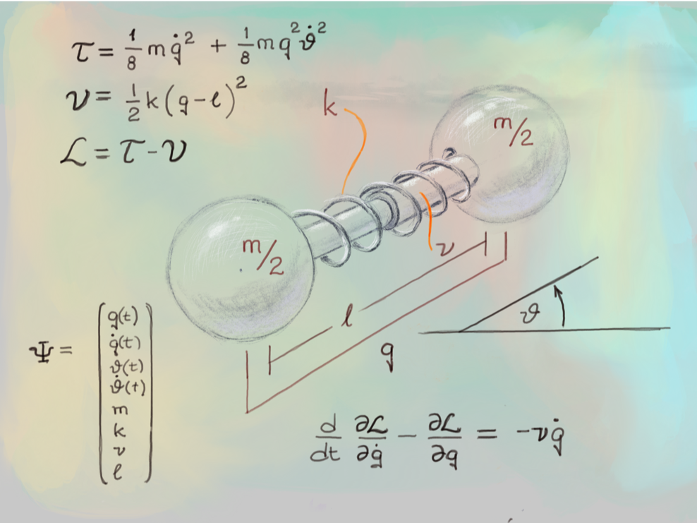
The system is illustrated in the following figure, wherein is the mass distributed in two weights at the end of a spring with spring constant , resting (zero-energy) length , and damping constant (Greek “nu”). These are parameters we’re going to measure by observing the system “in-flight.” The kinetic energy , potential energy , Lagrangian , state-space form , and the Euler-Lagrange equations for dynamics are written in longhand in the figure.
m
k
l
ν
ℒ
Ψ
Setup
Setup
The 2D problem has two degrees of freedom: extension of the spring and angle with respect to the horizontal axis of the inertial (free-fall) frame. Let be the distance between two equal masses . Let the origin of frame be the center of the bar. Each mass moves with speed with respect to that origin.
q
θ
q
m/2
q'[τ]/2
The kinetic energy as a function of time τ is
In[]:=
T=+++
1
2
m
2
2
-q'[τ]
2
m
2
2
q'[τ]
2
1
2
m
2
2
-q[τ]
2
m
2
2
q[τ]
2
2
θ'[τ]
Out[]=
1
8
2
′
q
1
8
2
q[τ]
2
′
θ
The conjugate momenta are
In[]:=
{pq[τ],pθ[τ]}(D[T,#]&/@{q'[τ],θ'[τ]})
Out[]=
{pq[τ],pθ[τ]}m[τ],m[τ]
1
4
′
q
1
4
2
q[τ]
′
θ
The Lagrangian velocities, in terms of the Hamiltonian variables, are:
In[]:=
hams=Solve[%,{q'[τ],θ'[τ]}]
Out[]=
[τ],[τ]
′
q
4pq[τ]
m
′
θ
4pθ[τ]
m
2
q[τ]
Therefore, the kinetic energy, in Hamiltonian terms, is
In[]:=
T/.First[hams]
Out[]=
2
2
pq[τ]
m
2
2
pθ[τ]
m
2
q[τ]
The potential energy, for both the Lagrangian and the Hamiltonian, with the resting length, , a constant, is
l
In[]:=
V=k
1
2
2
(q[τ]-l)
Out[]=
1
2
2
(-l+q[τ])
The dissipative force on each mass is half the total, so the total, for the Lagrangian, is
In[]:=
f=-νq'[τ]
Out[]=
-ν[τ]
′
q
For the Hamiltonian, it is
In[]:=
f/.First[hams]
Out[]=
-
4νpq[τ]
m
The Lagrangian equations of motion follow here. Note that they are computed symbolically, for reliability, via Wolfram’s derivative operator, (it’s too easy to make a mistake by hand, even with a tiny system like this one).
D
In[]:=
With[{Lcrds={q[τ],θ[τ]}},With[{Lvels=D[Lcrds,τ],L=T-V},With[{Lncnf={-ν,0}*Lvels},Leqns=Flatten@MapThread[{q,v,h}D[D[L,v],τ]-D[L,q]h,{Lcrds,Lvels,Lncnf}]//FullSimplify]]]
Out[]=
{4kl+mq[τ][τ]4kq[τ]+4ν[τ]+m[τ],mq[τ](2[τ][τ]+q[τ][τ])0}
2
′
θ
′
q
′′
q
′
q
′
θ
′′
θ
The Hamiltonian equations of motion are more compact and devoid of puns between the second argument of and the time derivatives of generalized coordinates:
q
ℒ
In[]:=
With{Hcrds={q[τ],θ[τ]},Hmoms={pq[τ],pθ[τ]},H=(T+V)/.First[hams]},WithHncnf=-,0*Hmoms,Flatten@MapThread[{q,p,f}{D[H,q]f-D[p,τ],D[H,p]D[q,τ]},{Hcrds,Hmoms,Hncnf}]//FullSimplify
4ν
m
Out[]=
+kq[τ]+[τ]kl+,[τ],[τ]0,[τ]
4νpq[τ]
m
′
pq
4
2
pθ[τ]
m
3
q[τ]
′
q
4pq[τ]
m
′
pθ
4pθ[τ]
m
2
q[τ]
′
θ
State-Space Form
State-Space Form
The forms above are suitable for numerical integration of ground truth via built-in integrators (last section of the notebook). We need symbolic forms for derivations below.
State Vector
State Vector
In[]:=
Ψ=
;
q |
qdot |
θ |
θdot |
m |
k |
ν |
l |
Exact System Dynamics
Exact System Dynamics
We employ exact dynamics to generate fake observations as well as for ground truth.
Lagrangian equations of motion in state-space form:
In[]:=
Solve[Leqns,{q''[τ],θ''[τ]}]//FullSimplify
Out[]=
[τ],[τ]-
′′
q
4kl-4kq[τ]-4ν[τ]+mq[τ][τ]
′
q
2
′
θ
m
′′
θ
2[τ][τ]
′
q
′
θ
q[τ]
These equations are non-linear in the components of the state vector. Write them in affine form for subsequent linearization in the Extended Kalman Filter (EKF):
In[]:=
ClearAll[symRules];symRules[ψ_,x_]:=Flatten@Quiet@
;
ψ〚1,1〛x〚1,1〛 |
ψ〚2,1〛x〚2,1〛 |
ψ〚3,1〛x〚3,1〛 |
ψ〚4,1〛x〚4,1〛 |
ψ〚5,1〛x〚5,1〛 |
ψ〚6,1〛x〚6,1〛 |
ψ〚7,1〛x〚7,1〛 |
ψ〚8,1〛x〚8,1〛 |
Initial Conditions
Initial Conditions
Integration
Integration
The following integrator can handle dynamics that depend explicitly on time, even though dynamics in this application do not depend explicitly on time.
TODO: partially evaluate or lambda lift over Dx (exact non-linear dynamics). No reason to keep passing that in.
Verification
Verification
Reproduce ground-truth extracted ex-post-facto from the bottom “ground-truth” section of the notebook. This is not exactly cheating. Instead, it amounts to iteration-to-convergence of the entire exercise.
Prediction (System Dynamics)
Prediction (System Dynamics)
This section assumes proficiency with the Extended Kalman Filter. See Zarchan and Musoff or Bruce Gibbs for background.
The Fundamental Matrix
The Fundamental Matrix
The exact, nonlinear dynamics have the form
Start with the Jacobian of the exact dynamics:
Sanity-check the integration with the following, first-order recurrence:
“Regularize” the fundamental matrix by hacking out the offending term:
The following is just plotting code. No interesting dynamics here.
Propagator
Propagator
Process Noise
Process Noise
Update (Observation Model)
Update (Observation Model)
Observation Partials
Observation Partials
Observation Noise
Observation Noise
Observation noise is a function of state and time that returns a covariance matrix in the same units as the observations, denoted Capital Zeta, Ζ. Lambda lift over constant parameters of the noise distribution because this is the common case.
TODO: Verify the aero-drag models in [KF5] with this more general form of the EKF.
Observation Partials (Revisited)
Observation Partials (Revisited)
Observation Noise (Revisited)
Observation Noise (Revisited)
Synthetic Data
Synthetic Data
Let the observed angle vary from ground truth by an unbiased normal variate of ten degrees.
EKF
EKF
Without comments:
Experiments
Experiments
The following will occasionally overflow if you set parameters to high-hazard values. That’s on purpose, precisely so you may explore the parameter spaces. If the experiment produces messages, just tweak a parameter so that it runs again.
The checkboxes indicate which variables and parameters are estimated from the data. An unchecked box causes the corresponding a‑priori covariance to be zero, meaning “the observations are 100% correct.” The sliders let you change observation noise, process noise, and overall multiplier for the covariance. Overall, the system behaves as expected, but there are some interesting scenarios to explore.
Finally, check all the boxes and see that the system-identified parameters tend to converge to their a‑priori values. In this case, the EKF is estimating everything available and the statistical constraints are perhaps too strong.
Play around with this, and perhaps you’ll find these techniques useful in your own system-identification work.
Ground Truth
Ground Truth
The following method constructs and solves the equations of motion directly from the Lagrangian and Hamiltonian. It does not require the equations of motion separately. It produces approximately the same results as the rk4 accumulator above, just with more sophisticated integration techniques encapsulated in NDSolve.
References
References
[KF5] Kalman Folding 5: Non-Linear Models and the EKF, Brian Beckman, https://vixra.org/abs/1607.0084
Zarchan and Musoff
Fundamentals of Kalman Filtering: A Practical Approach (Progress in Astronautics and Aeronautics, 232) 3rd Edition
by Paul Zarchan (Author), Howard Musoff (Author), Frank K. Lu (Editor), https://a.co/d/eq8UQwv
Fundamentals of Kalman Filtering: A Practical Approach (Progress in Astronautics and Aeronautics, 232) 3rd Edition
by Paul Zarchan (Author), Howard Musoff (Author), Frank K. Lu (Editor), https://a.co/d/eq8UQwv
Bruce Gibbs
Advanced Kalman Filtering, Least-Squares and Modeling: A Practical Handbook 1st Edition
by Bruce P. Gibbs (Author), https://a.co/d/daxGy12
Advanced Kalman Filtering, Least-Squares and Modeling: A Practical Handbook 1st Edition
by Bruce P. Gibbs (Author), https://a.co/d/daxGy12
CITE THIS NOTEBOOK
CITE THIS NOTEBOOK
Bottle-Flip System Identification by Kalman Filtering
by Brian Beckman
Wolfram Community, STAFF PICKS, February 11, 2024
https://community.wolfram.com/groups/-/m/t/3120367
by Brian Beckman
Wolfram Community, STAFF PICKS, February 11, 2024
https://community.wolfram.com/groups/-/m/t/3120367