This project investigates the influence of quantum noise on the performance of quantum algorithms. Simple quantum noise models are explored theoretically in both single-qubit and multi-qubit systems. First, we will simulate a 1-qubit quantum circuit with a noise channel, studying how the nature and magnitude of the noise can be characterized and estimated using only measurement counts. The results of these simulations will be applied to measurements performed on quantum processing units (QPUs) to characterize the effects of quantum noise in real quantum computing hardware.
Introduction
Introduction
Noise in the quantum computing
Noise in the quantum computing
Quantum computers utilize different physical realizations of logical qubits. Whether the hardware is based on superconducting circuits, trapped ions, or Rydberg atoms, the system is always exposed to interactions with the environment. The macroscopic manifestation of quantum phenomena can be easily perturbed by thermal noise, vibrations, and instrument imperfections. Quantum mechanics predicts numerous effects that can affect the performance of a quantum computer. The uncertainty principle and zero-point fluctuations result from the principles of quantum mechanics, and their influence on a quantum system is referred to as quantum noise. The main effect of performing quantum computations in a noisy environment is the decoherence of a quantum state. As noise causes the loss of superposition, which is the very thing that marks quantum supremacy in computing, understanding its nature seems to be the crucial challenge in the field of quantum computing.
The goal of that project is to explore the nature of the quantum noise using Quantum Framework of the Wolfram Language:
Installation of the Quantum Framework paclet:
In[]:=
PacletInstall["https://wolfr.am/DevWQCF",ForceVersionInstall->True]Needs["Wolfram`QuantumFramework`"]
Out[]=
PacletObject

BitFlip noise
BitFlip noise
The simplest model of noise in the quantum circuit is bit flip. It’s the channel that with certain probability applies NOT gate to the logical qubit.
In[]:=
$Assumptions=Element[θ,Reals]&&Element[ϕ,Reals]&&Element[p,Reals]&&1>p>0psi={Cos[θ/2],Sin[θ/2]};
Iϕ
E
Out[]=
θ∈&&ϕ∈&&p∈&&1>p>0
Theoretical expression for probability of measuring state . Initial state is given by . The bit flip channel is used with probability parameter p:
|0〉
cos
θ
2
|0〉+sin
ϕ
θ
2
|1〉
In[]:=
qcBitFlipTheory=QuantumCircuitOperator[{QuantumState[psi],"BitFlip"[p]}];predictionBitFlip=qcBitFlipTheory[]["Probabilities"][[1]]//Simplify
Out[]=
1
2
Simulating the measurement
Simulating the measurement
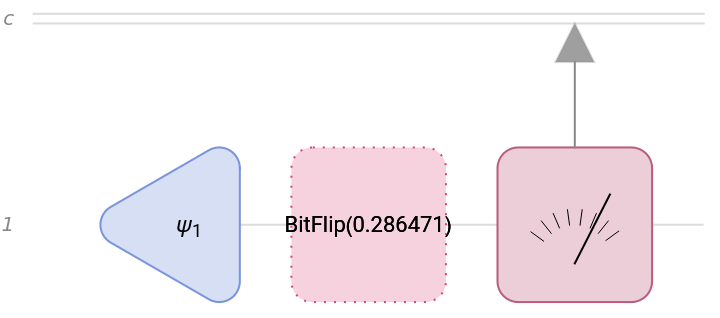
To simulate a real measurement parameter p=0.2 is set and the random noise is added.
In[]:=
qcBitFlipMeasurement=QuantumCircuitOperator[{QuantumState[psi],"BitFlip"[0.2+RandomReal[{0.0,0.1}]],"M"}];qcBitFlipMeasurement["Diagram"]
Out[]=
In[]:=
measureBitFlip[θ_]:=QuantumCircuitOperator[{QuantumState[psi/.ϕ->0],"BitFlip"[0.2+RandomReal[{0.0,0.1}]],"M"}][]["ProbabilitiesList"][[1]];measurementsBitFlip=Table[{θ,measureBitFlip[θ]},{θ,0.0,Pi,0.1}];
Analysis
Analysis
To retrieve the information about the noise channel and the value of parameter p one can fit function (1 + Cos(θ) - 2p Cos(θ)) to simulated/measured data.
1
2
In[]:=
fitBitFlip=FindFit[measurementsBitFlip,predictionBitFlip,p,θ]
Out[]=
{p0.243987}
In[]:=
Show[ListPlot[measurementsBitFlip,AxesLabel->{"θ","Probability"},PlotLegends->Placed[{"Simulation"},{Right,Top}],ImageSizeLarge],Plot[predictionBitFlip/.fitBitFlip,{θ,0.0,Pi},PlotStyle->Red,PlotLegends->Placed[{"Theory"},{Right,Top}],ImageSizeLarge]]
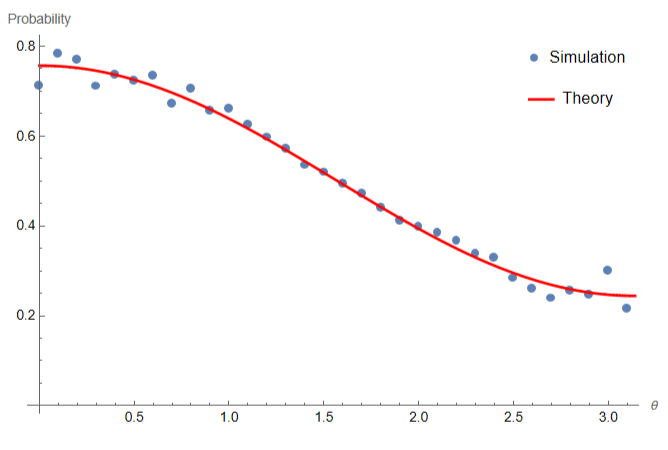
The form of the fitted function tells us that the noise channel is indeed a bitflip channel. This approach will be applied to data from the real hardware.
General noise model
General noise model
In a more general case noise channel consists of matrix made of 4 free parameters applied with certain probability p.
In[]:=
$Assumptions=Element[θ,Reals]&&Element[ϕ,Reals]&&Element[p,Reals]&&1>p>0&&Element[a,Reals]&&Element[b,Reals]&&Element[c,Reals]&&Element[d,Reals]
Out[]=
θ∈&&ϕ∈&&p∈&&1>p>0&&a∈&&b∈&&c∈&&d∈
In[]:=
generalChannel=QuantumChannel[{
1-p
{{1,0},{0,1}},p
{{a,b},{c,d}}}];MatrixForm/@generalChannel["Tensor"]Out[]=
,
1-p | 0 |
0 | 1-p |
a p | b p |
c p | d p |
Theoretical expression for probability of measuring state |0〉. Initial state is given by :
cos
θ
2
|0〉+sin
ϕ
θ
2
|1〉
In[]:=
predictionGeneralNoise=QuantumCircuitOperator[{QuantumState[psi],generalChannel}][]["Probabilities"][[1]]//Simplify
Out[]=
Abs1+(-1+)p+bp2b+a(1+)Sin[θ]Absp+1+(-1+)p+cd(1+)pSin[θ]+Abs1+(-1+)p+bp2b+a(1+)Sin[θ]
2
a
2
Cos
θ
2
1
2
2
Sin
θ
2
-ϕ
2ϕ
2
c
2
Cos
θ
2
2
d
2
Sin
θ
2
1
2
-ϕ
2ϕ
2
a
2
Cos
θ
2
1
2
2
Sin
θ
2
-ϕ
2ϕ
Simulating the measurement
Simulating the measurement
Measurements are simulated by specifying values of parameters and slightly varying them by adding the noise.
In[]:=
measureGeneralNoise[θ_,ϕ_]:=Simplify/@QuantumCircuitOperator[{QuantumState[{Cos[θ/2],Sin[θ/2]}],QuantumChannel[{
Iϕ
E
1-p
{{1,0},{0,1}},p
{{a,b},{c,d}}}/.{p->0.3+RandomReal[{0.0,0.1}],a->2.+RandomReal[{0.0,0.1}],b->3.+RandomReal[{0.0,0.1}],c->1.+RandomReal[{0.0,0.1}],d->4.+RandomReal[{0.0,0.1}]}]}][]["Probabilities"][[1]];In[]:=
measurementsGeneralNoise=Table[{{θ,ϕ},measureGeneralNoise[θ,ϕ]},{θ,0.0,Pi,0.2},{ϕ,0.0,2Pi,0.5}];
In[]:=
measurementsGeneralNoisePhi0=Table[{θ,measureGeneralNoise[θ,0.]},{θ,0.0,Pi,0.1}];
Analysis
Analysis
Probability distribution for measuring state dependent on values of θ and ϕ on the Bloch sphere:
|0〉
In[]:=
interpolationProbabilityGeneralNoise=Interpolation[Flatten[measurementsGeneralNoise,1]]
Out[]=
InterpolatingFunction

In[]:=
Quiet[plot2=SphericalPlot3D[1,{θ,0,π},{Φ,0,2π},ColorFunction->Function[{x,y,z,θ,Φ,r},ColorData["Rainbow"][interpolationProbabilityGeneralNoise[θ,Φ]]],PlotPoints->100,ColorFunctionScaling->False,Mesh->False,Boxed->False,AxesFalse,ImageSize->Medium];]Row[{plot2,BarLegend["Rainbow"]}]
The probability function is fitted to simulated measurement data and values of parameters p, a ,b ,c and d can be obtained.
IBM measurements
IBM measurements
Example of measurement
Example of measurement
Results from IBM Kyoto
Results from IBM Kyoto
Results from IBM Osaka
Results from IBM Osaka
Concluding Remarks
Concluding Remarks
Further research
Further research
Research can be extended to a 2-qubit system. Assuming that bitflip is the dominant type of noise, its influence on the results could vary with different levels of entanglement. Moreover, investigating the time dependence of measurement accuracy in such a system can reveal differences between the nature of quantum and classical noise.
Acknowledgments
Acknowledgments
The project was completed during Wolfram Summer School 2024. I’d like to express my gratitude to my mentors: Mads Bahrami, Paul Abbott, Bruno Tenorio, and Sebastian Rodriguez for their invaluable help.
I want to thank the Dean for Students’ Affairs of the Faculty of Physics at the University of Warsaw, Krzysztof Turzyński, who made my participation in WSS possible.
I want to thank the Dean for Students’ Affairs of the Faculty of Physics at the University of Warsaw, Krzysztof Turzyński, who made my participation in WSS possible.
References
References
1
.S.Devitt et al. (2013), “Quantum error correction for beginners” Rep. Prog. Phys. 76 076001
2
.Cite This Notebook
Cite This Notebook