ABSTRACT (original article): Phenological mismatch has been highlighted as a reason why climate change is causing declines of migratory populations. The likelihood of declines due to phenological mismatch might depend on what cues trigger migration. Migrants that use environmental cues (e.g. temperature, resource availability) to trigger migration are often considered to be less vulnerable than migrants that use temporal information (e.g. photoperiod). We developed a proof-of-concept model that demonstrates that which cue type performs better in the context of phenological change can depend on differences in seasonal amplitude between the habitats used by a migrant. Environmental cues perform better than temporal cues when the habitat that undergoes a phenological change has a larger seasonal amplitude. This result aligns with observations that populations of short-distance migrants that use environmental cues are less likely to decline as a consequence of phenological mismatch than long-distance avian migrants that use temporal cues. Temporal cues perform better than environmental cues when the habitat that undergoes a phenological change has a smaller seasonal amplitude. This result may correspond to empirical scenarios where the more seasonal habitat is associated with variation in precipitation patterns or human actions that are not changing in phenology. In addition to these results, we offer distinctions that will help clarify future work on phenological mismatch. First, we highlight the difference between the cue accuracy (difference between the timing of migration using the cue and optimal migration timing) and the cue efficacy (the difference between the fitness using the cue and the fitness using optimal migration). Second, we recommend considering both how the benefits available from migrating and the benefits that are captured by migrants change with phenological change. CITATION (original article): Torstenson, M. and Shaw, A.K. (2024), Strength of seasonality and type of migratory cue determine the fitness consequences of changing phenology for migratory animals. Oikos e10862. https://doi.org/10.1111/oik.10862
Equal amplitude habitat quality functions
Equal amplitude habitat quality functions
In this model, migrants move between habitats in which the habitat quality varies as a function of time . We begin by exploring the case in which the two habitat quality functions have the same amplitude .
ClearAll["Global'*"]
Before phenological change
Before phenological change
We explore optimal migration before phenological change.
The original habitat quality functions are given by
The original habitat quality functions are given by
In[]:=
H1[x_]:=Sin[x]H2[x_,b_]:=Sin[x-b]
If migration takes no time and has no costs, then optimal migration occurs whenever the habitat functions cross. The x values of the points at which the functions cross can be thought of as a time cue of optimal migration. We calculate the values of the time cues for optimal migration. We want values on the interval 0<=b<=2Pi.
In[]:=
H=Solve[{H1[x]==H2[x,b],0<=b<=2Pi,0<=x<=3Pi},x,Reals]
Out[]=
x,x,x,x
In[]:=
t1=Values[Normal[H[[1]],ConditionalExpression]]t2=Values[Normal[H[[2]],ConditionalExpression]]t3=Values[Normal[H[[3]],ConditionalExpression]]t4=Values[Normal[H[[4]],ConditionalExpression]]
Out[]=
b-π
2
Out[]=
b+π
2
Out[]=
(b+3π)
1
2
Out[]=
(b+5π)
1
2
We then calculate the y values at which optimal migration occurs. These can be thought of as habitat quality cues of optimal migration.
In[]:=
hcue1=FullSimplifySin
b-π
2
Out[]=
-Cos
b
2
In[]:=
hcue2=FullSimplifySin
b+π
2
Out[]=
Cos
b
2
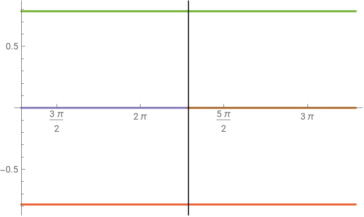
We can visualize how the benefit of migration depends on b and where the time and habitat quality cues occur in this interactive figure. The blue sine curve is the habitat quality function of habitat 1. The orange sine curve is the habitat quality function of habitat 2. The shaded areas represent the cumulative experienced habitat quality. The horizontal lines are the habitat quality cues and the vertical lines are the time cues. We start and end the annual cycle with a migration from habitat 1 to habitat 2.
ManipulatePlotH1[x],H2[x,b],-Cos,Cos,ConditionalExpression0,<=x<=,ConditionalExpression0,<=x<=,x,,,,{b,0,2Pi}
b
2
b
2
b+π
2
b+3π
2
b+3π
2
b+5π
2
b+π
2
b+5π
2
Out[]=


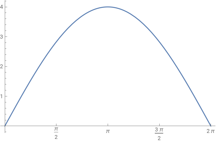
We can now calculate how the total experienced habitat quality over the course of a year varies as a function of b when migration occurs at optimal times.
In[]:=
Eo=FullSimplify[Integrate[H2[x,b],{x,t2,t3}]+Integrate[H1[x],{x,t3,t4}]]Plot[{Eo},{b,0,2*Pi},Ticks->{Range[0,2Pi,Pi/2],Automatic}]
Out[]=
4Sin
b
2
Out[]=
We can also calculate the benefit of migration, that is, how much more habitat quality is experienced over the annual cycle than would have been if the migrant stayed in one of the habitats year round. Note that this is equal to the total experienced benefit because the integral of y=sin(x-b) over the interval x ∈ [0,2π] is 0 for all b.
Bo=Eo-Integrate[H1[x],{x,t2,t4}]
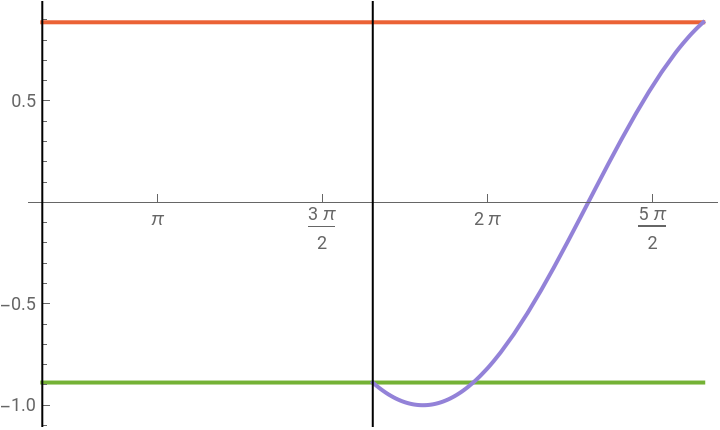
Using the same format as the interactive plot above, we can visualize the benefit of migration as the area between the habitat 1 and habitat 2 curves during the interval when the migrant is in habitat 1.
ManipulatePlotH1[x],H2[x,b],-Cos,Cos,ConditionalExpressionSin[x-b],<=x<=,x,,,,{b,0,2Pi}
b
2
b
2
b+3π
2
b+5π
2
b+π
2
b+5π
2
Out[]=
After phenological change
After phenological change
We now implement a horizontal shift in the habitat quality function of habitat 2 to represent phenological change.
In[]:=
H2N[{x_,b_,c_}]:=Sin[x-b-c]
Migration using time cues that were previously optimal occurs at the same times as were calculated above. We calculate when migration using previously optimal habitat quality cues will now occur.
In[]:=
t1h=Values[Normal[Solve[{H1[x]==Sin[t2],Sin'[x]<0,0<=b<=Pi,0<=x<=2Pi},x,Reals],ConditionalExpression]]
Out[]=
b+π
2
In[]:=
t2h=Values[Normal[Solve[{H2N[{x,b,c}]==Sin[t3],Derivative[{1,0,0}][H2N][{x,b,c}]<0,0<=b<=Pi,0<=c<=Pi,Pi<=x<=2Pi},x,Reals],ConditionalExpression]]
Out[]=
(b+2c+3π)
1
2
We now calculate the total experienced habitat quality and benefit of migration following phenological change using previously optimal time cues.
In[]:=
Et=Simplify[Integrate[H2N[{x,b,c}],{x,t2,t3}]+Integrate[H1[x],{x,t3,t4}]]Bt=Et-Integrate[H1[x],{x,t1h,t1h+2*Pi}]
Out[]=
2Sin+Sin+c
b
2
b
2
Out[]=
2Sin+Sin+c
b
2
b
2
We also calculate the total experienced habitat quality and benefit of migration following phenological change using previously optimal habitat quality cues.
In[]:=
Eh=Simplify[Integrate[H2N[{x,b,c}],{x,t1h,t2h}]+Integrate[H1[x],{x,t2h,t1h+2*Pi}]]
Out[]=
4CosSin
c
2
b+c
2
In[]:=
Bh=Eh-Integrate[H1[x],{x,t1h,t1h+2*Pi}]
We then calculate the difference between the benefit of migration following phenological change using previously optimal time or habitat quality cues and find that it is zero, meaning that the two cue types function equally well following phenological change.
We plot the new benefit of migration using either cue as a function of b (x axis) and c (y axis)
We also calculate the difference in the habitat quality experienced before and after phenological change for both cue types and plot it as a function of b (x axis) and c (y axis)
Finally, we calculate and plot the difference between the benefit of migration that is available and the benefit received following phenological change for both cue types.
Different amplitude habitat quality functions
Different amplitude habitat quality functions
We now explore the case where the two habitat quality functions have different amplitudes. The new initial habitat quality functions are given by...
We solve by hand for the optimal migration times and find that they take the form t=arctan(sin (b)/(cos(b)+a))+Pi*Z where Z is an integer. If we want the annual cycle to start near t=0, then they can the following 4 forms depending on a and b
We initialize the annual cycle at some time t such that it is an optimal time for migration from habitat 1 to habitat 2 and end the annual cycle at time t+2Pi. There are some conditions under which this t is t1 and others under which this time is t2.
We now solve for the optimal habitat quality cues. This requires the exploration of two different conditions.
Condition 1: start in Habitat 2 at time t1, migrate to habitat 1 at time t2 and migrate back to habitat 2 at time t1+2Pi. This condition applies when
1a) a <1 and 0<b mod 2Pi< ArcCos(a)
1b) a <1 and 2Pi-ArcCos(a)< b mod 2Pi <=2Pi
Condition 2: start in Habitat 2 at time t2, migrate to habitat 1 at time t3 and migrate back to Habitat 2 at time t2+2 Pi. This condition applies when
2a) a>=1
2b) a <1 and ArcCos(a)<b<2Pi-ArcCos(a))
Now, given condition 1 is met, the initial optimal habitat quality cues occur at
Given condition 2 is met, the initial optimal habitat quality cues occur at
We can visualize the habitat quality experienced in this case by looking at the the integral under the curve in the habitat where the migrant is given migration times represented by the vertical lines and habitat cues are represented by horizontal lines. Note that the sliders may not work for the edge cases - just slide them a little bit.
We can visualize the habitat quality experienced in this case by looking at the the integral under the curve in the habitat where the migrant is given migration times represented by the vertical lines and habitat cues are represented by horizontal lines. Note that the sliders may not work for the edge cases - just slide them a little bit.
We now calculate the original experienced habitat quality . Note that because migration occurs at the same times in both conditions, but for any given time at which a migrant goes from habitat 2 to habitat 1 in condition 1, it will go from habitat 1 to habitat 2 in condition 2, (and vice versa), and because optimal migration always leads to positive habitat quality, the original experienced habitat quality can be expressed as the absolute value of that which is calculated for either condition .
One difference in the case where the habitat quality functions have different amplitudes is that migration can have a non-zero benefit when b=0. We show this by setting b=0 in the above equations and simplifying.
We can also interactively visualize the initial benefit of migration using sliders. Note that sliders may not work for edge cases.
(*Condition 1a*)
We now plot the initial benefit of migration as a function of a and b (density plot - a on x axis, b on y axis). As in the equal amplitudes case, note that this is equal to the experienced habitat quality.
After phenological change
After phenological change
We now implement a horizontal shift in the habitat quality function of habitat 2 to represent phenological change .
We go on to explore the consequences of phenological change when previously optimal time vs. habitat quality based cues are used.
Temporal cues
Temporal cues
We start by calculating the experienced habitat quality after phenological change when previously optimal time cues are used.
We plot experienced habitat quality using previously optimal habitat quality cues on a density plot as a function of a (on y axis) and c(on x axis) when b=pi. Note that when b=Pi we are always in condition 2.
We also plot the new experienced habitat quality using sliders to allow b (the x axis) to vary in addition to a and c (sliders).
We also plot new benefit of migration as the area between curves.
We go on to calculate the difference between the benefit of migration before and after phenological change when time based cues are used.
We plot difference from original experienced habitat quality when time based cues are used as a function of a (y axis) and c (x axis) as a density plot where b=Pi. (*Note that when b=Pi, we are always in condition 2*)
We also plot difference from original experienced habitat quality using sliders to allow b (the x axis) to vary in addition to a and c (sliders).
We also calculate difference between available benefit and benefit received following phenological change(available - received) (*Note that sometimes adding c will switch which condition we are in for the benefit available*)
Habitat quality cues
Habitat quality cues
We now turn our attention to the consequences of phenological change when previously optimal habitat quality cues are used .
We begin by identifying when migration using previously optimal habitat quality cues occurs.
We begin by identifying when migration using previously optimal habitat quality cues occurs.
(*Condition 1*)
Note that because the Habitat 1 function does not change,the initial migration from 1 to 2 occurs at...
and the final migration from Habitat 1 to Habitat 2 occurs at
We now solve for the migration from Habitat 2 to habitat 1 that occurs between these values
Note that these solutions are mod 2Pi. The values that can work on the interval we are interested in are...
We note that we want to pick the habitat quality cue such that the habitat cue when c=0 is equal to the time cue, which is at t2 in condition 1 - Recall that t2 = ArcTan[Sin[b]/(Cos[b]-a)]+Pi *). We find that for condition 1, this happens at one of three potential time values -
1.1) when b=Pi (and when b is sufficiently close to Pi) the appropriate habitat quality cue timing always occurs at b+c+ArcSin[Sin[b+ArcCot[(a-Cos[b]) Csc[b]]]]. Note that this condition is not met in condition 1a or 1b.
1.2) For a <=1 (one of the requisites for condition 1) when a is sufficiently small and b is sufficiently close to 0 on the interval b = 0 to 2Pi (as in condition 1a), the appropriate habitat quality cue timing occurs at b+π-ArcSin[Sin[b+ArcCot[(a-Cos[b]) Csc[b]]]]
1.3) when a is sufficiently small and b is sufficiently close to 2 Pi on the interval b= 0 to 2Pi (as in condition 1b) the appropriate habitat quality cue timing occurs at b+c-π-ArcSin[Sin[b+ArcCot[(a-Cos[b]) Csc[b]]]]*)
(*Condition 2*)
Note that because Habitat 1 is not moving, the initial migration from 1 to 2 occurs at...
and the final migration from Habitat 1 to Habitat 2 occurs at...
We now solve for the migration from Habitat 2 to habitat 1 that occurs between these values
Note that either of these solutions are mod 2Pi. The values that could work on the interval we are interested in are...
Note that, as above, we want to pick the cue such that the habitat cue when c=0 is equal to the time cue, which is at t3 in condition 2. Recall that t3 = ArcTan[Sin[b]/(Cos[b]-a)]+2Pi. This occurs at one of three times.
2.1 When b = Pi/ b is sufficiently close to Pi (as is generally true in conditions 2 b and 2 c and sometimes true in 2a), this always occurs at b+c+π+ArcSin[Sin[b+ArcCot[(a-Cos[b]) Csc[b]]]]
2.2 When b is sufficiently close to zero on the interval b= 0 to 2 Pi, this occurs at b+c-ArcSin[Sin[b+ArcCot[(a-Cos[b]) Csc[b]]]] (sometimes true in 2a)
2.3 When b is sufficiently close to 2Pi on the interval b= 0 to 2 Pi, this occurs at b+c+2Pi-ArcSin[Sin[b+ArcCot[(a-Cos[b]) Csc[b]]]] (sometimes true in 2a)
We can now calculate experienced habitat quality when previously optimal habitat quality cues are used.
We now plot experienced habitat quality when using previously optimal habitat quality cues as a density plot when b=Pi as a function of a (y axis) and c (x axis). Because b = Pi, we only plot condition 2.1.
We also plot the new experienced habitat quality using sliders to allow b (the x axis) to vary in addition to a and c (sliders) . Note that these graphs only apply for the range of a,b,c values for which the condition is appropriate.
We also plot new benefit of migration as the area between curves.
We display these plots for cases in which the migrant starts in Habitat 2 at time t2, migrating to habitat 1 at time t3 and migrating back to Habitat 2 at time t2+2 Pi . This applies when
2a) a>=1
2b) a <1 and Pi<b<2Pi-ArcCos(a))
2c) a<1 and ArcCos(a)<b<=Pi mod 2Pi*)
We display these plots for cases in which the migrant starts in Habitat 2 at time t2, migrating to habitat 1 at time t3 and migrating back to Habitat 2 at time t2+2 Pi . This applies when
2a) a>=1
2b) a <1 and Pi<b<2Pi-ArcCos(a))
2c) a<1 and ArcCos(a)<b<=Pi mod 2Pi*)
We now calculate the difference from the original experienced habitat quality when habitat quality cues are used
We can now plot difference from original experienced habitat quality when habitat quality cues are used as a function of a (y axis) and c (x axis) as a density plot where b= Pi. This means that condition 2.1 applies.
Comparing time and habitat quality cues
Comparing time and habitat quality cues
To compare the performance of the two cue types, we calculate difference between habitat quality experienced following phenological change when the migrant uses previously optimal time or habitat quality cues.
We now plot the difference between habitat quality experienced using time and habitat quality cues as a function of a (x axis)and c (y axis) as a density plot where b=pi.
CITE THIS NOTEBOOK
CITE THIS NOTEBOOK
Seasonality and migratory cues shape fitness impacts of phenological shifts in migratory species
by Martha Torstenson and Allison K. Shaw
Wolfram Community, STAFF PICKS, November 20, 2024
https://community.wolfram.com/groups/-/m/t/3325199
by Martha Torstenson and Allison K. Shaw
Wolfram Community, STAFF PICKS, November 20, 2024
https://community.wolfram.com/groups/-/m/t/3325199