In[]:=
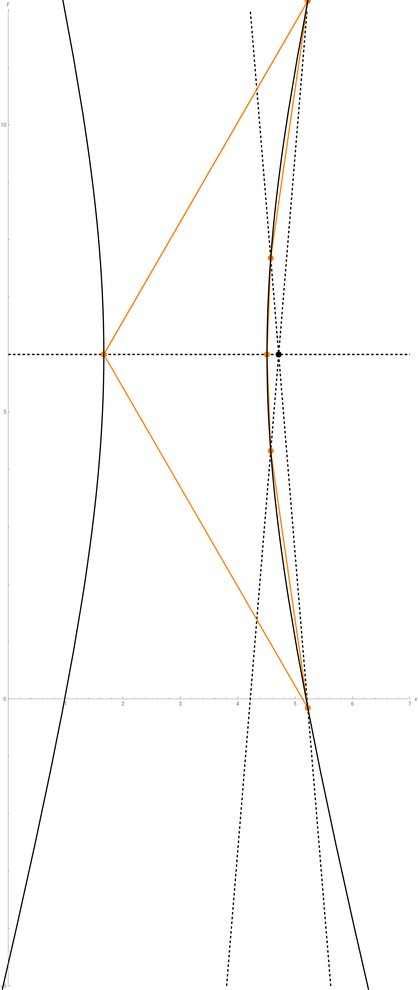
BrianchonTheorem::usage="It states that, given a hexagon circumscribed on a conic section, the lines joining opposite polygon vertices (polygon diagonals) meet in single point.Reference:WolframMathWorld:Brianchon'sTheorem;Personal";
The following animation verifies the theorem:
In[]:=
ManipulateShowr=2;k=4;d=-3;n=6;ρ=;x1=4;y1=6;TableGraphicsBlack,Dashed,Thick,InfiniteLine{4-d,y1}++-{(r+ρ)Cos[t1+2πk1]+x1-(4-d),(r+ρ)Sin[t1+2πk1]+y1-6},{4-d,y1}++-{(r+ρ)Cos[t1+2πk1+π]+x1-(4-d),(r+ρ)Sin[t1+2πk1+π]+y1-6},t1,0,2π,,TableGraphicsOrange,PointSize[0.015],Point{4-d,y1}++-{(r+ρ)Cos[t1+2πk1]+x1-(4-d),(r+ρ)Sin[t1+2πk1]+y1-6},t1,0,2π,,TableGraphicsOrange,Thick,Line{4-d,y1}++-{(r+ρ)Cos[t1+2πk1]+x1-(4-d),(r+ρ)Sin[t1+2πk1]+y1-6},{4-d,y1}++-(r+ρ)Cost1++2πk1+x1-(4-d),(r+ρ)Sint1++2πk1+y1-6,t1,0,2π,,ParametricPlotCosh[t]+,Sinh[t]+6,{t,-π,π},PlotStyle->{Black,Thick},ParametricPlot-Cosh[t]+,Sinh[t]+6,{t,-π,π},PlotStyle->{Black,Thick},GraphicsBlack,PointSize[0.015],Point,6,AxesTrue,AxesLabel{x,y},BoxRatiosAutomatic,AxesOrigin{0,0},ImageSize700,PlotRange{{0,7},{-5,12}},Style["Brianchon's Theorem:",Bold,Large],{{k1,0,"Valor (k1)"},0,6,0.2},ControlPlacementTop
2Sin
π
n
1-Sin
π
n
2
k
2
((r+ρ)Cos[t1+2πk1]+x1-(4-d))
2
((r+ρ)Sin[t1+2πk1]+y1-6)
2
ρ
2
k
2
((r+ρ)Cos[t1+2πk1+π]+x1-(4-d))
2
((r+ρ)Sin[t1+2πk1+π]+y1-6)
2
ρ
2π
n
2
k
2
((r+ρ)Cos[t1+2πk1]+x1-(4-d))
2
((r+ρ)Sin[t1+2πk1]+y1-6)
2
ρ
2π
n
2
k
2
((r+ρ)Cos[t1+2πk1]+x1-(4-d))
2
((r+ρ)Sin[t1+2πk1]+y1-6)
2
ρ
2
k
2
(r+ρ)Cost1++2πk1+x1-(4-d)
2π
n
2
(r+ρ)Sint1++2πk1+y1-6
2π
n
2
ρ
2π
n
2π
n
2π
n
128
90
139
45
64
3
15
128
90
139
45
64
3
15
33
7
Out[]=