In the following example we will illustrate how to apply the quantum natural gradient descent optimization for parametrized quantum circuits by calculating the Fubiny–Study metric tensor through different approaches.
Paclet Installation
Paclet Installation
Wolfram quantum framework is a paclet. So first, let’s install it:
PacletInstall["https://wolfr.am/DevWQCF",ForceVersionInstall->True]
<<Wolfram`QuantumFramework`
Theory
Theory
An optimization step in a gradient descent is given by:
θ
t+1
θ
t
where ℒ(θ) is the cost function with parameters θ, and η is the step rate. Each step in this approach assumes a flat Euclidean space, which would lead us to not–unique parametrizations that can disrupt our optimization, specially in singular points. In order to avoid this problem we must use non-Euclidean parameter spaces, performing what is called a natural gradient descent.
The quantum state space features an invariant metric tensor referred to as the Fubini–Study metric tensor , which can be used to develop a quantum version of a natural gradient descent. Then each optimization step is given by:
g
ij
θ
t+1
θ
t
+
g
where the Fubini-Study metric tensor pseudo-inverse.
+
g
In the following example we will demonstrate two methods to calculate the Fubini–Study metric tensor:
◼
Using the cost function indistinguishability in a variational quantum eigensolver setting.
◼
Using a block–diagonal approximation.
In both cases we will perform a natural gradient optimization and compare it with classical methods.
Variational quantum eigensolver (VQE)
Variational quantum eigensolver (VQE)
The fundamental process of the Variational Quantum Eigensolver (VQE) involves using a brief quantum circuit U(θ), characterized by parameters θ = , . . . ,}, to iteratively adjust θ to minimize the average energy or cost function: for the ansatz .
{
θ
1
θ
m
f(θ)=〈ϕ(θ)|H|ϕ(θ)〉
|ϕ(θ)〉=U(θ)|0〉
In the VQE setting the Fubiny-Study metric follows:
g
ij
∂
i
∂
j
∂
i
ϕ
ϕ
∂
j
where
|ϕ(θ)〉=|ϕ(θ)〉/∂.
∂
i
∂
i
θ
i
Block-diagonal metric tensor
Block-diagonal metric tensor
We can calculate using an approximation of the Fubini-Study metric tensor for a variational quantum circuit, named the block-diagonal approach:
g
(l)
g
ij
ψ
l-1
K
i
K
j
ψ
l-1
ψ
l-1
K
i
ψ
l-1
ψ
l-1
K
j
ψ
l-1
The circuit is given by:
U(θ)|〉=()...()...()|〉
ψ
0
V
L
θ
L
W
L
V
l
θ
l
W
l
V
0
θ
0
W
0
ψ
0
where W are layers of non-parametrized gates and are the generators of the parametrized gates V of the form .
(l)
K
i
(l)
θ
i
(l)
K
i
The quantum state before the application of layer l is:
|〉=()...()|〉
ψ
l-1
V
l-1
θ
l-1
W
l-1
V
0
θ
0
W
0
ψ
0
Defining Helper Functions
Defining Helper Functions
Single qubit example
Single qubit example
We can solve a single qubit example using VQE algorithm. We need to drive the following ansatz state to the ground state of the Hamiltonian
H=
σ
x
In[]:=
singleState=QuantumState[{Cos[θ1],Exp[2*I*θ2]*Sin[θ1]},"Parameters"->{θ1,θ2}];singleState["Formula"]
Out[]=
Cos[θ1]|0〉+Sin[θ1]|1〉
2θ2
Fubini-Study metric tensor calculation
Fubini-Study metric tensor calculation
Following the theory, we can implement a function to calculate the Fubini-Study metric tensor from a state:
|ϕ(θ)〉
We will need the correspondent ϕ ket and bra. Since it is a simple exam\bple, we will use fancy notation for our variables:
In[]:=
|ϕ〉=singleState["StateVector"];
In[]:=
〈ϕ|=singleState["Dagger"]["StateVector"];
Follow the equation for ={,}
Reϕϕ-ϕϕ
∂
i
∂
j
∂
i
ϕ
ϕ
∂
j
θ
i
θ
1
θ
2
In[]:=
singleStateFubini[{θ1_,θ2_}]=Table[Re[D[〈ϕ|,θi].D[|ϕ〉,θj]]-D[〈ϕ|,θi].|ϕ〉〈ϕ|.D[|ϕ〉,θj],{θi,{θ1,θ2}},{θj,{θ1,θ2}}]//Normal//ComplexExpand//FullSimplify;singleStateFubini[{θ1,θ2}]//MatrixForm
Out[]//MatrixForm=
1 | 0 |
0 | 2 Sin[2θ1] |
Cost function
Cost function
Let’s calculate the energy (cost) function:
In[]:=
singleStateCost[θ1_,θ2_]=〈ϕ|.PauliMatrix[1].|ϕ〉;singleStateCost[θ1,θ2]//ComplexExpand//FullSimplify
Out[]=
Cos[2θ2]Sin[2θ1]
Proceed to calculate the correspondent gradient for each :
θ
i
In[]:=
singleStateCostGrad[θ1_,θ2_]=Grad[singleStateCost[θ1,θ2],{θ1,θ2}]//ComplexExpand//Simplify
Out[]=
{2Cos[2θ1]Cos[2θ2],-8Cos[θ1]Cos[θ2]Sin[θ1]Sin[θ2]}
Test using θ1=π/12andθ2=π/12
Test using =π/12and=π/12
θ
1
θ
2
For our gradient descent and quantum gradient descent we will be using GradientDescent and QuantumNaturalGradient functions, with for 50 steps:
η=0.05
singleStateQuantumParameters=QuantumNaturalGradientDescent[{π/12,π/12},0.05,singleStateFubini,singleStateCostGrad,50];
In[]:=
singleStateVainillaParameters=GradientDescent[{π/12,π/12},0.05,singleStateCostGrad,50];
Let’s plot our variables and their correspondant cost function to compare the optimization steps:
Out[]=
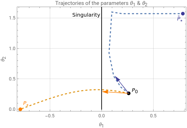


Analyzing the trajectory we discover that the Natural Gradient Descent gets as optimum point closest to the point ={-π/4,0}. The main issue is that the line =0 is a singular point and depending on the metric, it may cause the distance to change. In the other hand, the Quantum Natural Gradient Descent gets as optimum point closest to the point ={π/4,π/2} which does not cross the singular point.
P
0
P
*
θ
1
P
0
P
*
In[]:=
ListLinePlot[{singleStateCost@@@singleStateQuantumParameters,singleStateCost@@@singleStateVainillaParameters},PlotRange->All,PlotLegends->{"Quantum Natural Gradient Descent","Gradient Descent"},FrameLabel->{"Optimization steps","Cost Function Value"},Frame->True,GridLines->Automatic]
Out[]=
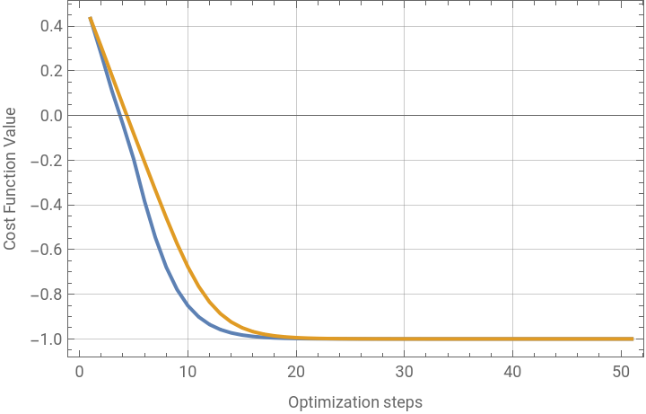


The ground state is reached in less steps by the quantum gradient descent.
Test using θ1=5π/12andθ2=π/12
Test using =5π/12and=π/12
θ
1
θ
2
In[]:=
singleStateQuantumParameters2=QuantumNaturalGradientDescent[{5π/12,π/12},0.05,singleStateFubini,singleStateCostGrad,50];
In[]:=
singleStateVainillaParameters2=GradientDescent[{5π/12,π/12},0.05,singleStateCostGrad,50];
Out[]=
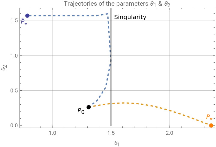
As the previous example, now the singularity is found at =π/2. The quantum descent result is the same as the last example, the regular algorithm fails to notice the singularity.
θ
1
In[]:=
ListLinePlot[{singleStateCost@@@singleStateQuantumParameters2,singleStateCost@@@singleStateVainillaParameters2},PlotRange->All,PlotLegends->{"Quantum Natural Gradient Descent","Gradient Descent"},FrameLabel->{"Optimization steps","Cost Function Value"},Frame->True,GridLines->Automatic]
Again, the ground state is reached in less steps by the quantum gradient descent.
Variational Quantum Circuit example
Variational Quantum Circuit example
Circuits & State
Circuits & State
Let’s build a “more complicated” circuit for the following example:
Block-diagonal implementation
Block-diagonal implementation
Consider the following variational quantum circuit
Step-by-step calculation
Step-by-step calculation
In this case we got 2 parametrized layers with two parameters each, then following the block-diagonal approach:
Calculate the first layer using the following formula:
The second layer:
Then the block diagonal matrix is the following:
Acknowledgment
Acknowledgment
I would like to express my sincere gratitude to Cesar Guerra and the Wolfram Quantum Computation Framework Team for their help through this notebook implementation.
References
References
Yamamoto, N. (2019). On the natural gradient for variational quantum eigensolver (Version 1). arXiv. https://doi.org/10.48550/ARXIV.1909.05074
Izaac, J. (2019). Quantum natural gradient. PennyLane Demos. https://pennylane.ai/qml/demos/tutorial_quantum_natural_gradient/
CITE THIS NOTEBOOK
CITE THIS NOTEBOOK
Natural gradient descent optimization for quantum circuits with Fubiny–Study metric tensor
by Sebastian Rodriguez
Wolfram Community, STAFF PICKS, February 28, 2024
https://community.wolfram.com/groups/-/m/t/3131997
by Sebastian Rodriguez
Wolfram Community, STAFF PICKS, February 28, 2024
https://community.wolfram.com/groups/-/m/t/3131997