We study phase transitions in the transverse field Ising Model using the Quantum Framework Paclet. We compute the mean magnetization and the entanglement entropy for up to =12 qubits. At zero temperature, we confirm the existence of a second order phase transition when the ratio of the spin-spin interaction and the external magnetic field parameter is unity. The mean magnetization is shown to vanish as the coupling to the external magnetic field is large. The entanglement entropy is computed numerically and compared against known results. The numerical study shows the central charge which is close to the expected result of
n
q
c≈.518
c1/2.
The Quantum Transverse Field Ising Chain
The Quantum Transverse Field Ising Chain
Background
Background
The Ising model is perhaps the most well recognized model in condensed matter and statistical physics described by the Hamiltonian where are classical spins on a -dimensional spatial lattice with a binary output and corresponding to nearest neighbor spin interactions. The above Hamiltonian for the classical Ising model is related to to the quantum transverse field Ising model (TFIM) on a -dimensional spatial lattice formed out of qubits
H=-
J
∑
<i,j>
S
i
S
j
S
i
(d+1)
{-1,1}
<i,j>
d
H=-J⊗+h
∑
<i,j>
z
σ
i
z
σ
j
∑
i
x
σ
i
via the transfer matrix method. Here are the Pauli spin operators with eigenstates {|↓〉, 〈↑} and eigenvalues respectively and operates on these states by spin flip. The external field appears from the duality mapping to a lower dimension.
In fact, the TFIM can be seen as a special case of the Heisenberg model known as the XXZ model. The relationship between the classical and quantum coupling parameters↔(J,h) is explored in this blog post.
Here, the purpose is to study the quantum TFIM chain and calculate the mean magnetization as a function of the coupling, i.e., , and the entanglement entropy. For simplicity, we set henceforth.
σ
{-1,1}
x
σ
h
In fact, the TFIM can be seen as a special case of the Heisenberg model known as the XXZ model. The relationship between the classical and quantum coupling parameters
J
Here, the purpose is to study the
1d
M(h)
J=1
Code
Code
Here, I build the Hamiltonian matrix in the eigenbasis for an arbitrary long quantum Ising chain as a function of the external field strength . First, let’s load the paclet.
z
σ
h
In[]:=
PacletInstall[CloudObject["https://wolfr.am/DevWQCF"],ForceVersionInstall->True]<<Wolfram`QuantumFramework`
Out[]=
PacletObject

Boundary Conditions
Boundary Conditions
One can either choose periodic (pbcs = True)or antiperiodic boundary conditions(pbcs = False)depending on the problem. If the following value is set to be true, then the last Ising spin will interact with the first.
In[]:=
pairlist[n_]:=If[periodicboundaryconditions,Join[Partition[Range[n],2,1],{{n,1}}],Partition[Range[n],2,1]]
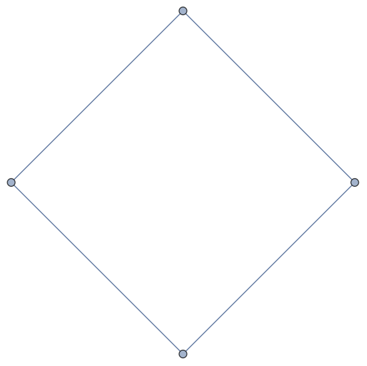
As an example, this is how the spin interactions look like in a =4 qubit interaction:
n
q
In[]:=
{Evaluate[periodicboundaryconditions=False];Graph[pairlist[4]],Evaluate[periodicboundaryconditions=True];Graph[pairlist[4]]}
Out[]=
,

For the rest of this discussion, I set this condition to be True.
periodicboundaryconditions=True
Hamiltonian
Hamiltonian
In[]:=
hamiltonian[n_,h_]:=hamiltonian[n,h]=-Total[QuantumOperator["Z",#]&/@pairlist[n]]-hTotal@Table[QuantumOperator["X",{i}],{i,n}]
Let’s check the matrix representation of the Hamiltonian in a =3 qubit model
n
q
In[]:=
"ℋ[3,h] = "MatrixForm[hamiltonian[3,h]["Matrix"]]
Out[]=
ℋ[3,h] =
-2 | -h | -h | 0 | -h | 0 | 0 | 0 |
-h | 0 | 0 | -h | 0 | -h | 0 | 0 |
-h | 0 | 2 | -h | 0 | 0 | -h | 0 |
0 | -h | -h | 0 | 0 | 0 | 0 | -h |
-h | 0 | 0 | 0 | 0 | -h | -h | 0 |
0 | -h | 0 | 0 | -h | 2 | 0 | -h |
0 | 0 | -h | 0 | -h | 0 | 0 | -h |
0 | 0 | 0 | -h | 0 | -h | -h | -2 |
Ground State
Ground State
Next, the ground state is found by choosing the eigenvector associated with the largest negative magnitude eigenvalue of the quantum Ising chain. This is computationally expensive for large qubit number ≫1.
n
q
In[]:=
Nq=12;(*ThisvaluesetsthenumberofqubitsintheIsingchain*)
In[]:=
hValues=Flatten[Prepend[N[Table[,{i,-2,2,1/2}]],{0}]];
i
10
In[]:=
ClearAll[eigenvals,eigenvecs]
In[]:=
eigenvals=SparseArray[{},{Nq-1,Length[hValues]}];
In[]:=
eigenvecs=SparseArray[{},{Nq-1,Length[hValues]}];
In[]:=
Table[Table[({eigenvals[[j-1,i]],eigenvecs[[j-1,i]]}=Eigensystem[N[hamiltonian[j,hValues[[i]]]["Matrix"]],2]),{i,1,Length[hValues]}],{j,2,Nq}];
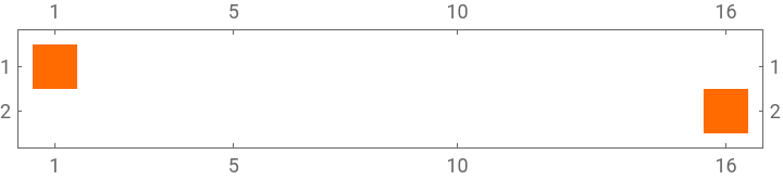
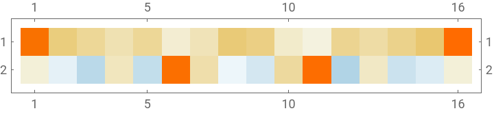
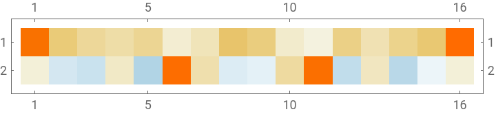
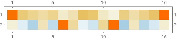
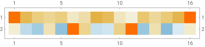
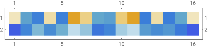
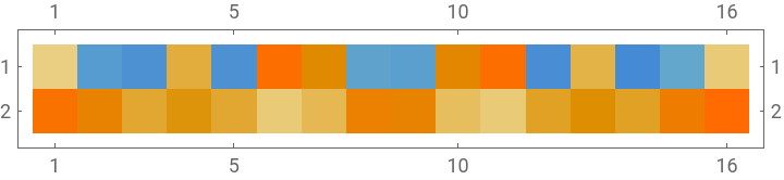
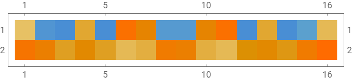
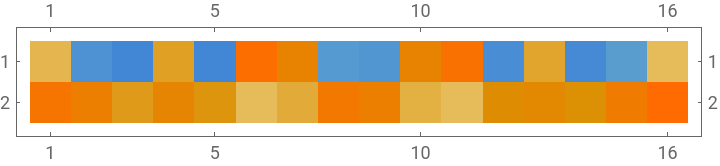
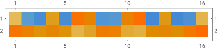
Let' s look at the first two ground state eigenvectors for 4 qubits with in the given domain.
h
In[]:=
MatrixPlot/@eigenvecs[[3]]
Out[]=
,
,
,
,
,
,
,
,
,
In[]:=
groundstates=Table[Table[First[eigenvecs[[j-1,i]][[First[Position[Ordering[eigenvals[[j-1,i]]],1]]]]],{i,1,Length[hValues]}],{j,2,Nq}];
Let's check if the ground state and corresponding eigenvalue we calculated is indeed consistent with the Hamiltonian acting on ground state vector. For =3 qubits without an external field,
n
q
In[]:=
hamiltonian[3,0]["Matrix"].groundstates[[2,1]]==eigenvals[[2,1,1]]*groundstates[[2,1]]
Out[]=
True
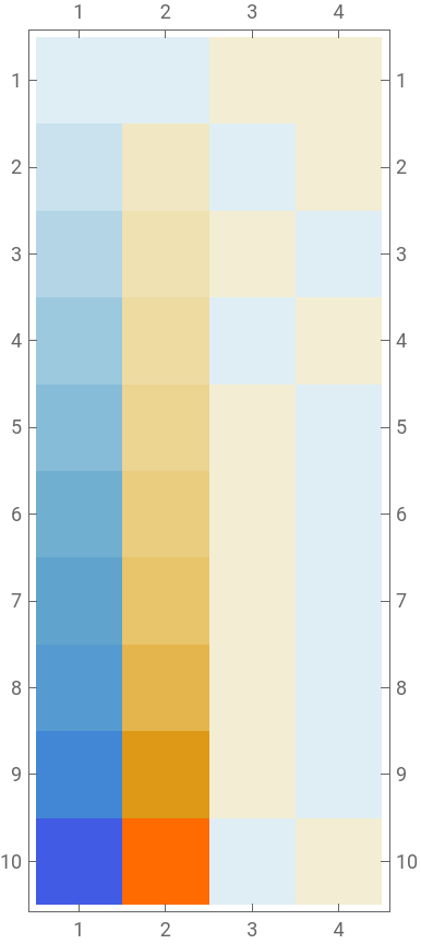
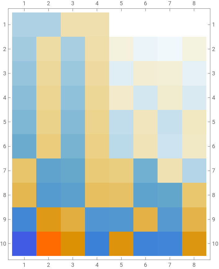
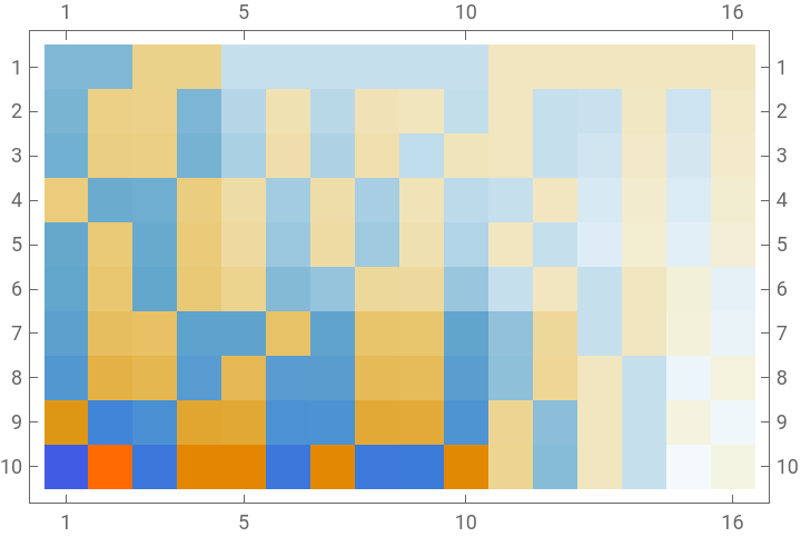
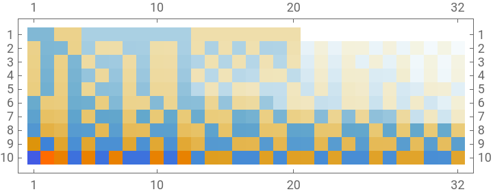
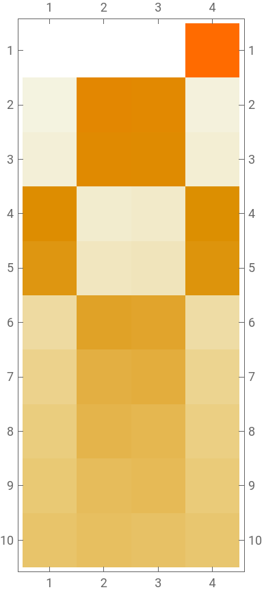
we see that indeed the ground state is an eigenstate of the Hamiltonian. We can visualize the eigenvalues and eigenvectors
In[]:=
Table[MatrixPlot[Table[Eigenvalues[hamiltonian[j,hValues[[i]]]["Matrix"]],{i,1,Length[hValues]}]],{j,2,5}]
Out[]=
,
,
,
In[]:=
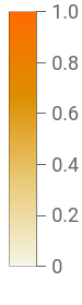
MatrixPlot[Table[,{i,1,Length[hValues]}],PlotLegendsAutomatic]
2
Abs[Eigenvectors[hamiltonian[2,hValues[[i]]]["Matrix"]][[1]]]
Out[]=
Mean Magnetization
Mean Magnetization
Lastly, the mean magnetization can be found by constructing a quantum operator, much like the Hamiltonian above, and then computing
Magnetization of the 12 Qubit Chain
Magnetization of the 12 Qubit Chain
Entanglement Entropy
Entanglement Entropy
One can also calculate directly the entanglement entropy stored in the system as a function of the magnetization. First, we need to convert each of the ground states vectors to be quantum ket states
4 Qubit Magnetization
4 Qubit Magnetization
Entanglement & Conformal Field Theory
Entanglement & Conformal Field Theory
Let’s study the 4 qubit chain and trace out up to 3 qubits and see if we can recover the CFT result.
Conclusions:
Conclusions:
References:
References:
1. Notes on the quantum/classical Ising duality: McGreevy UCSD Notes
2. Quantum Ising Phase Transition in JuliaPhysics
3. Review of Quantum Ising Models by Andrew Tan
2. Quantum Ising Phase Transition in JuliaPhysics
3. Review of Quantum Ising Models by Andrew Tan
Appendix: 12 Qubit Model
Appendix: 12 Qubit Model