Estimating Kinetic Parameters from a Batch Reactor Experiment
Authors: Housam Binous and Ahmed Bellagi
Estimating Kinetic Parameters from a Batch Reactor Experiment
Authors: Housam Binous and Ahmed Bellagi
Authors: Housam Binous and Ahmed Bellagi
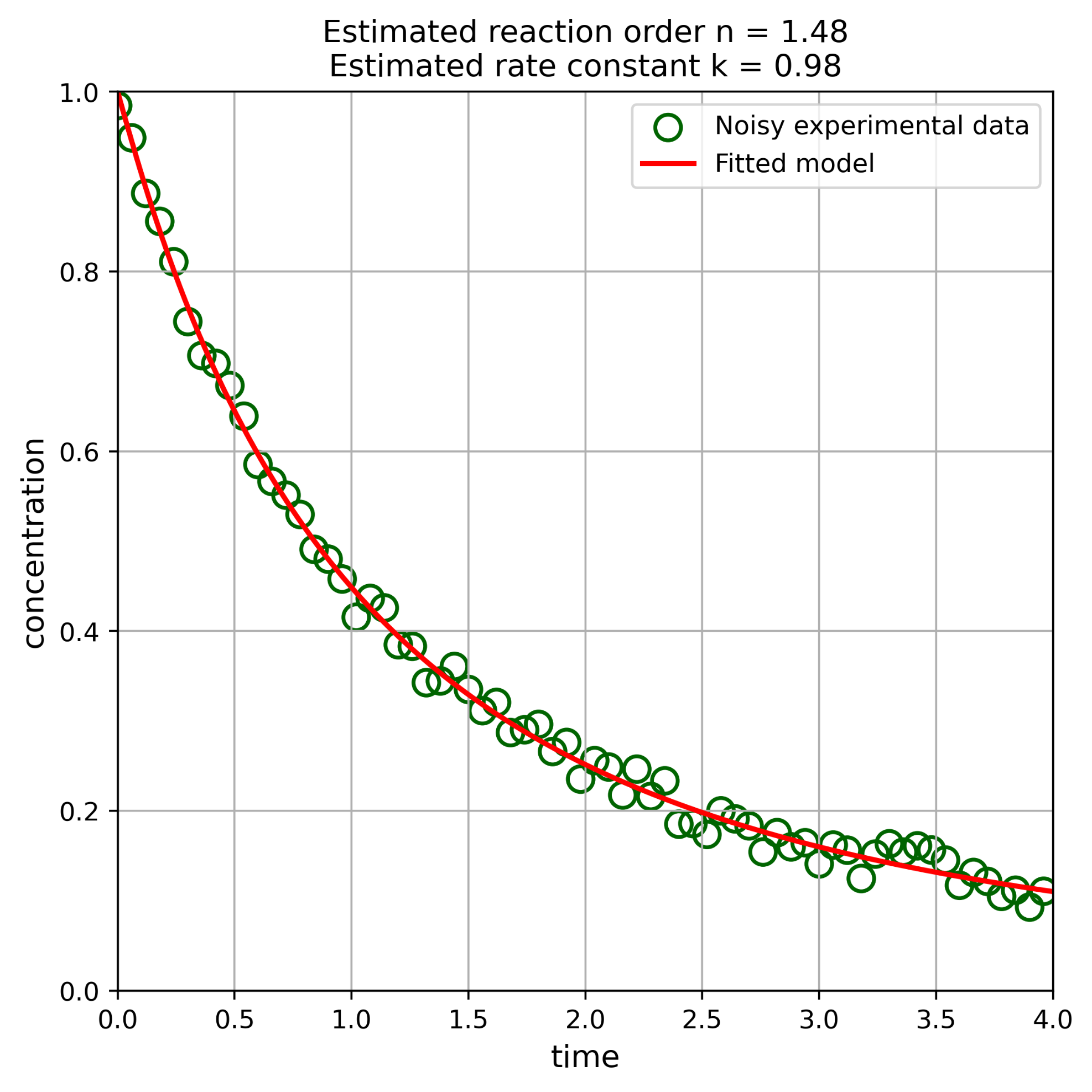
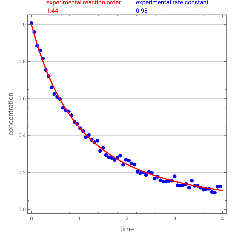
Consider an irreversible homogeneous liquid-phase reaction taking place in a batch reactor. Assume that the experimental data (i.e. the concentration of species versus time data indicated by the blue dots in the figure) comes from, for example, the on-line measurement of electrical conductivity of the mixture in the reactor. The governing equation of the batch reactor is given by =-k with .We use the experimentally obtained data in order to estimate the theoretical reaction order and rate constant (shown in the figure in red and blue, respectively). You can vary the theoretical values of and as well as the experimental data (in order to mimic different experimental results obtained by various set-ups using the “seed” and “noise amplitude” variables).Our result agree closely with its counterpart obtained using Python (Python coding is provided below). However, generating exactly the same noisy dataset is mathematically impossible across the two languages such as Mathematica and Python. Indeed, 1- Mathematica and NumPy use different random number generators, 2- NDSolve and solve_ivp use different numerical ODE solvers, and 3- Floating-point rounding and interpolation differ. However, as expected, the two languages yield very close estimates for the reaction order and rate constant .Finally, the methodology used here is fully documented in Ref. 1.References:[1] Mejri, S, Binous, H, Mahgoub, K, Bellagi, A. A model parameter estimation method using Mathematica© applied to transient chemical engineering processes, Comput Appl Eng Educ. 2018; 26 : 1405– 1421.
nAB
A
dc
dt
n
c
c(t=0)=1
n
k
n
k
n
k
In[]:=
n=1.5;(*reactionordern*)k=1;(*rateconstantk*)noise=0.05;(*noiseamplitude*)seed=1234;(*seedforrandomnumbergenerator*)
In[]:=
sol=NDSolve[{c'[t]-kc[t]^n,c[0]1},c,{t,0,10}];(*truesolution*)
In[]:=
SeedRandom[seed];noisydata=Table[{i,Max[0,First[noise(2Random[]-1)/2+c[t]/.sol/.ti]]},{i,0,4,0.06}];(*syntheticdatageneratedusingthetruesolutionandanoise*)
In[]:=
noisydata
Out[]=
{{0.,1.00906},{0.06,0.960307},{0.12,0.886601},{0.18,0.861552},{0.24,0.816696},{0.3,0.755421},{0.36,0.720941},{0.42,0.662198},{0.48,0.625909},{0.54,0.610469},{0.6,0.598055},{0.66,0.55186},{0.72,0.537191},{0.78,0.53079},{0.84,0.511392},{0.9,0.474453},{0.96,0.463699},{1.02,0.440712},{1.08,0.424943},{1.14,0.391098},{1.2,0.404013},{1.26,0.37704},{1.32,0.36477},{1.38,0.373285},{1.44,0.31735},{1.5,0.334482},{1.56,0.295884},{1.62,0.283526},{1.68,0.280196},{1.74,0.269641},{1.8,0.27952},{1.86,0.292564},{1.92,0.244591},{1.98,0.270725},{2.04,0.266247},{2.1,0.250517},{2.16,0.243888},{2.22,0.2046},{2.28,0.199074},{2.34,0.201098},{2.4,0.187199},{2.46,0.203942},{2.52,0.198214},{2.58,0.169023},{2.64,0.177991},{2.7,0.158268},{2.76,0.152097},{2.82,0.152349},{2.88,0.155836},{2.94,0.158149},{3.,0.180288},{3.06,0.133118},{3.12,0.130631},{3.18,0.134639},{3.24,0.138455},{3.3,0.120189},{3.36,0.15799},{3.42,0.128523},{3.48,0.129802},{3.54,0.120556},{3.6,0.108562},{3.66,0.112234},{3.72,0.113144},{3.78,0.0962226},{3.84,0.092706},{3.9,0.12443},{3.96,0.126069}}
In[]:=
p2=ListPlot[noisydata,JoinedFalse,PlotMarkersStyle["●",Blue,10],PlotRangeAll,FrameTrue,GridLinesAutomatic,AspectRatio1];
In[]:=
pfun=y/.ParametricNDSolve[{y'[t]-k1y[t]^n1,y[0]1},y,{t,0,10},{k1,n1},MaxStepsInfinity,Method"StiffnessSwitching"];fit=FindFit[noisydata,pfun[k1,n1][t],{{k1,1.0,2.0},{n1,1.5,2.0}},t];(*methodologybasedonParametricNDSolveandFindFitisthoroughlyexplainedinRef.1*)
In[]:=
p3=Plot[pfun[k1,n1][t]/.fit,{t,0,4},PlotRangeAll,FrameTrue,GridLinesAutomatic,AspectRatio1,PlotStyle{Thick,Red}];
In[]:=
Show[p2,p3,PlotRange{{0,4},{0,1}},ImageSize1.15×350{1,1},FrameLabel{Style["time",12],Style["concentration",12]},PlotLabelRow[{Style[Column[{"experimental reaction order",NumberForm[Chop@N@n1/.fit,{4,2}]}],Red]," ",Style[Column[{"experimental rate constant",NumberForm[Chop@N@k1/.fit,{4,2}]}],Blue]}]]
Out[]=
Pyhtoncodeandresults:
importnumpyasnpimportmatplotlib.pyplotaspltfromscipy.integrateimportsolve_ivpfromscipy.optimizeimportcurve_fit#===============================#1.PARAMETERS#===============================n_true=1.5#reactionorderk_true=1.0#rateconstantnoise_amp=0.05#noiseamplitudeseed=1234np.random.seed(seed)#===============================#2.TRUEODEMODEL#===============================defreaction_ode(t,c,k,n):return-k*c**n#SolveODEsol=solve_ivp(reaction_ode,[0,10],[1.0],args=(k_true,n_true),dense_output=True)#===============================#3.GENERATENOISYDATA#===============================t_data=np.arange(0,4.01,0.06)c_clean=sol.sol(t_data)[0]noise=noise_amp*(2*np.random.rand(len(t_data))-1)/2c_noisy=np.maximum(0,c_clean+noise)#===============================#4.MODELFORFITTING#===============================defmodel(t,k,n):sol=solve_ivp(reaction_ode,[0,max(t)],[1.0],args=(k,n),t_eval=t,method="LSODA")returnsol.y[0]#===============================#5.PARAMETERESTIMATION#===============================popt,pcov=curve_fit(model,t_data,c_noisy,p0=[1.0, 1],bounds=([0,0],[2.0,2.0]))k_fit,n_fit=poptprint(f"Estimated rate constant k = {k_fit:.4f}")print(f"Estimated reaction order n = {n_fit:.4f}")#===============================#6.FITTEDCURVE#===============================t_fit=np.linspace(0,4,300)c_fit=model(t_fit,k_fit,n_fit)#===============================#7.PLOTTING#===============================plt.figure(figsize=(6,6))plt.scatter(t_data,c_noisy,facecolors='none',#Nofill(opencircles)edgecolors='darkgreen',#Circlebordercolormarker='o',#Circlemarkers=100,#Markersizelinewidths=1.5,#Borderthicknesslabel='Noisyexperimentaldata')plt.plot(t_fit,c_fit,'r-',linewidth=2,label='Fittedmodel')plt.xlabel("time",fontsize=12)plt.ylabel("concentration",fontsize=12)plt.title(f"Estimated reaction order n = {n_fit:.2f}\n"f"Estimated rate constant k = {k_fit:.2f}",fontsize=12)plt.grid(True)plt.legend()plt.axis([0,4,0,1])plt.tight_layout()plt.show()