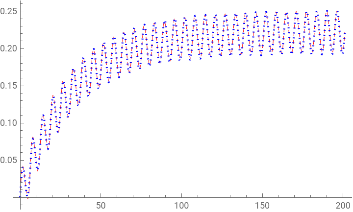
Start with the function of interest.
In[]:=
pmult=64;sol=NDSolveValue[{32f'[t]==Exp[Cos[t]-f[t]-f'[t]-f''[t]]-1,f[0]==0,f'[0]==0},f,{t,0,pmult*Pi},Method->{"EquationSimplification"->"Residual"}];Plot[sol[t],{t,0,pmult*Pi},PlotRange->All]
Out[]=
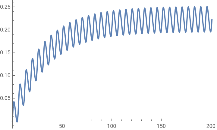
We' ll evaluate on a segment and stop well before this hits steady state.
In[]:=
obstime=30;timescale=1/10;start=0;dataM=Table[{t,sol[t]},{t,start,obstime,timescale}];len=Length[dataM];ListPlot[dataM]
Out[]=
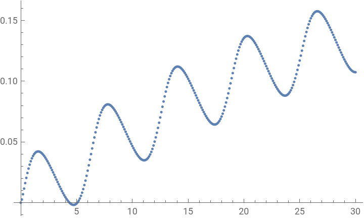
It appears that we have, to some approximation, a DC term, a damped exponential with negative coefficient and a sinusoid. So we’ll set up a model function of that form, and fit it to the data points.
In[]:=
model=a+b*Exp[t*c]+d*Sin[e*t];fit=FindFit[dataM,model,{a,b,c,d,e},t,Method->"NMinimize"]
Out[]=
{a0.228038,b-0.228288,c-0.0309627,d-0.0308703,e-0.999684}
This shows a steady-state mean around 0.228. Let’s check how well the fit matches the actual function.
In[]:=
p1=Plot[sol[t],{t,0,pmult*Pi},PlotRange->All,PlotStyle->Directive[Red,Thin,Dashed]];p2=Plot[model/.fit,{t,0,pmult*Pi},PlotRange->All,PlotStyle->Directive[Dotted,Blue]];Show[{p1,p2}]
Out[]=
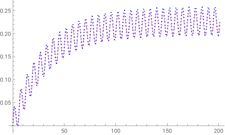
So we came fairly close, though it appears our fit goes a bit too high. If we used more data points we’d get a constant terms more in the vicinity of 0.222.
In[]:=
obstime=pmult/2*Pi;timescale=1/10;start=0;dataM=Table[{t,sol[t]},{t,start,obstime,timescale}];len=Length[dataM];ListPlot[dataM]
Out[]=
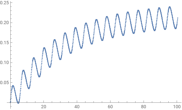
In[]:=
fit=FindFit[dataM,model,{a,b,c,d,e},t,Method->"NMinimize"]
Out[]=
{a0.221738,b-0.221642,c-0.0320042,d-0.0289715,e-0.999877}
In[]:=
p1=Plot[sol[t],{t,0,pmult*Pi},PlotRange->All,PlotStyle->Directive[Red,Thin,Dashed]];p2=Plot[model/.fit,{t,0,pmult*Pi},PlotRange->All,PlotStyle->Directive[Dotted,Blue]];Show[{p1,p2}]
Out[]=