Wolfram Cloud Document

This is part of live presentation series called Mathematical Games in which we explore a variety of games and puzzles using Wolfram Language. In this episode, we explore games with Markov chains or intransitivity.

demonstrations.wolfram.com

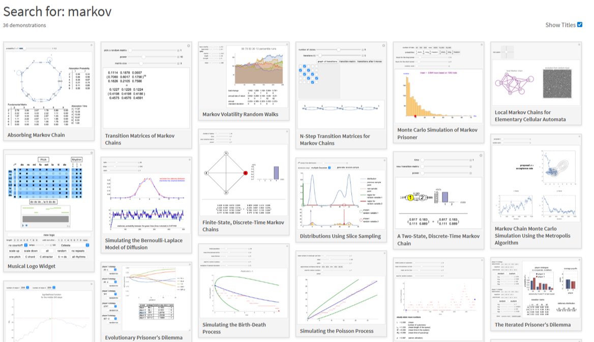
Many Demonstrations use Markov Chains.

The Original Experiment

In 1906, Andrey Markov wondered how letters followed each other in a piece of text. He used an obscure book by Pushkin, Eugene Onegin. Instead of that, we’ll use Alice in Wonderland. First, we’ll eliminate spaces and punctuation.

In[]:=

let=Characters["abcdefghijklmnopqrstuvwxyz"];alldoubles=Partition[Characters[ToLowerCase[ExampleData[{"Text","AliceInWonderland"}]]],2,1];double=SortBy[Tally[Select[alldoubles,MemberQ[let,#[[1]]]&&MemberQ[let,#[[2]]]&]],-Last[#]&];

Specifically, Markov wondered about how vowels and consonants followed each other.

In[]:=

vowels=Sort[{#[[1,1]],Total[#[[2]]]}&/@(Transpose/@GatherBy[{{If[MemberQ[Characters["aeiouy"],#[[1,1]]],"V","C"],If[MemberQ[Characters["aeiouy"],#[[1,2]]],"V","C"]},#[[2]]}&/@double,First])]

Out[]=

{{{C,C},6379},{{C,V},10803},{{V,C},9976},{{V,V},2119}}

Which would be these odds:

In[]:=

cv={"Con","Vowel"};vowelodds=#/Total[#]&/@Partition[Last/@vowels,2];Style[MatrixForm[N[vowelodds],TableHeadings->{cv,cv}],24]

Out[]=

	Con	Vowel
Con	0.371261	0.628739
Vowel	0.824804	0.175196

A chain of matrix multiplications might look like this:

Out[]=

6379 17182	10803 17182
9976 12095	2119 12095

6379 17182	10803 17182
9976 12095	2119 12095

6379 17182	10803 17182
9976 12095	2119 12095

6379 17182	10803 17182
9976 12095	2119 12095

6379 17182	10803 17182
9976 12095	2119 12095

If we raise the matrix to a power, we start getting a constant vector.

In[]:=

Style[MatrixForm[MatrixPower[vowelodds,10]//N],24]

Out[]=



0.567603	0.432397
0.567235	0.432765



It seems that the odds of the next letter being an consonant are .567

In[]:=

MatrixPower[vowelodds,100]//N

Out[]=

{{0.567444,0.432556},{0.567444,0.432556}}

Which is different than the original distribution:

In[]:=

letterodds=Transpose/@Reverse[GatherBy[Select[Tally[Characters[ToLowerCase[ExampleData[{"Text","AliceInWonderland"}]]]],MemberQ[Characters["abcdefghijklmnopqrstuvwxyz"],#[[1]]]&],MemberQ[Characters["aeiouy"],#[[1]]]&]];tots=Total[Last[#]]&/@letterodds;tots/Total[tots]//N

Out[]=

{0.595296,0.404704}

We can also include the punctuation:

In[]:=

CPV=If[MemberQ[let,#],If[MemberQ[Characters["aeiouy"],#],"V","C"],"P"]&/@Characters[ToLowerCase[ExampleData[{"Text","AliceInWonderland"}]]];allcharacters=#/Total[#]&/@Partition[Last/@Sort[Tally[Partition[CPV,2,1]]],3]

Out[]=



6379

23363

6181

23363

10803

23363

,

7008

12475

2507

12475

592

2495

,

9976

15883

3788

15883

2119

15883



Odds for the chance of following when punctuation is included:

In[]:=

vv={"Con","Punct","Vowel"};Style[MatrixForm[N[allcharacters],TableHeadings->{vv,vv}],24]

Out[]=

	Con	Punct	Vowel
Con	0.273039	0.264564	0.462398
Punct	0.561764	0.200962	0.237275
Vowel	0.628093	0.238494	0.133413

If we take a matrix power, we get a distribution for how things follow.

In[]:=

MatrixPower[allcharacters,100]//N

Out[]=

{{0.451711,0.241217,0.307072},{0.451711,0.241217,0.307072},{0.451711,0.241217,0.307072}}

This time, it’s similar to the distribution for single letters. Note: when I set this up, I didn’t know what the result would be. Scientific method and all that. Then again, Markov didn’t know either.

In[]:=

all=Last/@Sort[Tally[CPV]];N[all/Total[all]]

Out[]=

{0.451703,0.241213,0.307084}

Shuffling a Deck of Cards

In[]:=

ranks=Join[CharacterRange["2","9"],{"10","J","Q","K","A"}];suits={Style["♣",Black],Style["♠",Black],Style["♡",Red],Style["♢",Red]};deck=Row/@Tuples[{ranks,suits}];

In[]:=

deck

Out[]=

{2♣,2♠,2♡,2♢,3♣,3♠,3♡,3♢,4♣,4♠,4♡,4♢,5♣,5♠,5♡,5♢,6♣,6♠,6♡,6♢,7♣,7♠,7♡,7♢,8♣,8♠,8♡,8♢,9♣,9♠,9♡,9♢,10♣,10♠,10♡,10♢,J♣,J♠,J♡,J♢,Q♣,Q♠,Q♡,Q♢,K♣,K♠,K♡,K♢,A♣,A♠,A♡,A♢}

Perfect out-faro shuffle (top card stays on top):

In[]:=

outfaro=Riffle@@Partition[deck,Length@deck/2]

Out[]=

{2♣,8♡,2♠,8♢,2♡,9♣,2♢,9♠,3♣,9♡,3♠,9♢,3♡,10♣,3♢,10♠,4♣,10♡,4♠,10♢,4♡,J♣,4♢,J♠,5♣,J♡,5♠,J♢,5♡,Q♣,5♢,Q♠,6♣,Q♡,6♠,Q♢,6♡,K♣,6♢,K♠,7♣,K♡,7♠,K♢,7♡,A♣,7♢,A♠,8♣,A♡,8♠,A♢}

Perfect in-faro shuffle (top card moves to position 2):

In[]:=

infaro=Riffle@@Reverse@Partition[deck,Length@deck/2]

Out[]=

{8♡,2♣,8♢,2♠,9♣,2♡,9♠,2♢,9♡,3♣,9♢,3♠,10♣,3♡,10♠,3♢,10♡,4♣,10♢,4♠,J♣,4♡,J♠,4♢,J♡,5♣,J♢,5♠,Q♣,5♡,Q♠,5♢,Q♡,6♣,Q♢,6♠,K♣,6♡,K♠,6♢,K♡,7♣,K♢,7♠,A♣,7♡,A♠,7♢,A♡,8♣,A♢,8♠}

With eight perfect out-faro shuffles, the original deck is restored:

In[]:=

Nest[Riffle@@Partition[#,26]&,deck,8]

Out[]=

With 52 perfect in-faro shuffles, the original deck is restored:

In[]:=

Nest[Riffle@@Reverse@Partition[#,26]&,deck,52]

Out[]=

We need something sloppier than that for proper card mixing.

In[]:=

SloppyRiffle[deck_,slop_:1]:=Module[{n=Length@deck,half,drift,cut,a,b,side,out={},k,t},half=Ceiling[n/2];drift=If[slop==0,0,RandomVariate[SkellamDistribution[slop,slop]]];cut=Clip[half+drift,{1,n-1}];{a,b}=TakeDrop[deck,cut];side=RandomChoice[{Length@a,Length@b}->{1,2}];(*<--thisistheimportantfix*)While[a=!={}||b=!={},If[side==1&&a==={},side=2];If[side==2&&b==={},side=1];k=1+If[slop==0,0,RandomVariate[PoissonDistribution[slop]]];t=If[side==1,Take[a,UpTo[k]],Take[b,UpTo[k]]];out=Join[out,t];If[side==1,a=Drop[a,Length@t],b=Drop[b,Length@t]];side=3-side;];out]

Here’s a single sloppy shuffle

In[]:=

SloppyRiffle[deck,.3]

Out[]=

{2♣,8♡,8♢,2♠,2♡,9♣,2♢,9♠,9♡,3♣,9♢,3♠,10♣,3♡,10♠,10♡,3♢,10♢,4♣,J♣,4♠,J♠,4♡,J♡,4♢,J♢,5♣,Q♣,5♠,Q♠,5♡,Q♡,5♢,Q♢,6♣,K♣,6♠,K♠,6♡,K♡,6♢,K♢,7♣,A♣,A♠,7♠,7♡,A♡,7♢,A♢,8♣,8♠}

Do it a few times and the deck is mixed.

In[]:=

Nest[SloppyRiffle[#,.3]&,deck,5]

With sloppiness 0, the possible results are perfect in-faro and out-faro:

“Solomon W. Golomb, in his paper on “Permutations by Cutting and Shuffling,” proved that by mixing cuts with in-shuffles or with out-shuffles an even deck could reach any one of its possible permutations.” -- Martin Gardner, Mathematical Carnival.

Independently, Henri Poincaré devoted eight sections of his 1912 Calcul des Probabilités to card shuffling, an early motivation for random processes on finite sets/groups. The modern probabilistic riffle model used in math (Gilbert–Shannon–Reeds model, from a 1955 Bell Labs study, cut roughly in half then interleave with randomness) recommended seven shuffles for sufficient mixing and can be considered a Markov-chain model for human riffles. In 1992, Bayer & Diaconis verified seven shuffles.

Galton, 1873. English peerage.

How often do family lines die out?

Example

Tracing Card Paths during Perfect Shuffles (Adam Rumpf)

This Demonstration displays the path that each card takes through a deck over the course of a sequence of consecutive perfect shuffles. Each colored line traces the path of one card as a plot of position versus time. Use the controls to adjust the number of cards in the deck and whether the shuffle is an in-shuffle or an out-shuffle. The minimum number of shuffles required to return the deck to its original order is shown at the top.

Early Probability

Chebyshev inequality (1867): A bound on the probability that a random variable differs from its mean by more than a specified amount.

Markov inequality (1900): an upper bound on the probability that a random variable exceeds a positive constant.

Lyapunov inequality (1901): Higher moments of a random variable are at least as large, in a normalized sense, as lower moments.

Brownian Motion

In 1905 Einstein explained Brownian motion by treating a suspended particle as being buffeted by independent molecular kicks. From that he derived a quantitative prediction for diffusion. With D as the diffusion constant:

Brownian motion as a stochastic process arrived later with Wiener’s construction (1920s).
The axiomatic framework of probability by Kolmogorov came in 1933:
P1 (Nonnegativity): For any event A, P(A) ≥ 0. (probabilities can’t be negative)
P2 (Normalization): P(Ω) = 1. (something in the sample space must happen)
P3 (Countable additivity): If A1, A2, ... are pairwise disjoint, then P(⋃{i=1}^∞ Ai) = Σ{i=1}^∞ P(Ai).
(disjoint alternatives add, even for infinitely many)

One-Dimensional Fractional Brownian Motion (Roman E. Maeder)

Finding the Global Minimum of a Function Using Simulated Annealing (Housam Binous)

This Demonstration finds the global minimum of a function exhibiting several local minima. The method presented is based on simulated annealing, a numerical technique that rapidly determines the global minimum. The test function has the form:

((Simulated annealing is a Markov chain: each step proposes a random move from the current point and accepts it with a temperature-dependent probability.))

The Magic Octahedron

In this labeling of the octahedron, each vertex has edge-sum 26.

We can use this to randomly move around.

If you start on any vertex, after enough moves you have a 1/6th chance of being on any vertex.

A look at random walks:

We can approximate the distance from the origin after 1000 steps with the Maxwell distribution:

Asymmetric Magic Heptahedron

Here’s a magical heptahedron: all vertices have total edge-weight 24:

After a enough moves, the chance to be on any vertex is 1/7.

With a “magic” labeling, all the row sums and column sums add to one.
The matrix is doubly stochastic. As a result ... the odds are very fair.

Symmetry breaking

If one edge is directed, that’s enough to break the symmetry.

After repeated moves, you’re least likely to be on 1 (the source), and most likely to be on 3 (the sink):

We can get exact fractions for the behavior by using a high matrix power:

An easier method is to use the nullspace:

Weighted Digraph

Consider this graph. Puzzle: find a Hamiltonian cycle.

All Columns sum to 1.

After a few moves, the distribution for the vertices is far from balanced.

We can make a guess for most and least visited by summing the incoming values.

With nullspace, we can get the exact behavior, which is a bit different:

Absorbing Markov Chain (Conrad A. Benulis)

You can vary the probability of the transition from 2 to 1 with the slider. Because the sum of the probabilities is 1, for each state's total transitions, the transition probability for the transition from 2 to 3 is internally computed to sum to 1 when you drag the slider.

Penney Ante

A game by Walter Penney. Each player selects a series of head and tails.
Then a coin is flipped. Whoever’s sequence comes up first wins.
Barry Wolk supplied an analysis -- who also found magic labelings of graphs.

Penney Ante

We can recreate for the triples the probability of the Row winning.

And quadruples:

And quintuples

We can look at a developing pattern:

Level 5

We can look at the level 5 version.

Borel (1909) proved a strong law of large numbers for coin tossing. For IID (independent and identically distributed) Bernoulli trials X₁, X₂, … with Xₖ ∈ {0,1} and ℙ(Xₖ = 1) = p, the running mean X̄ₙ = (1/n) ∑_{k=1}^n Xₖ satisfies X̄ₙ → p almost surely (i.e. all infinite toss sequences except a probability-0 set).

In other words, if it’s a fair coin, with enough tosses, the results will converge to 1/2.

Coin Flips Demo (Non-transitivity)

In the ordered flip sequence HTTHHTHHHTHTTHHT, the four-flip sequence THHT occurs before HTHT. Two people could make a bet, each choosing a four-flip sequence, and then flip a coin until one of the sequences occurs. In the game, which sequence is best? Consider the two-flip sequences HH and TH. After three flips, the possibilities are HHH HHT HTH HTT THH THT TTH TTT. In these, HH appears first twice (HHH HHT), while TH appears first four times (HTH THH THT TTH).

This Demonstration shows how the four-flip sequences compare, with TTTT and HHHH left out, since neither is ever a good bet. Notice the counterclockwise ring of arrows on the outside—every flip sequence can win against at least one other. Thus, if you allow your victim to pick any sequence of four, you can always pick something better. For each pick, your best bet and the win fraction will be shown. Hover over other arrows to see their win rates.

Note: for 3 flips, you can’t get a non-transitive 6-cycle.

Dice Roll Sequences

With sequence of rolls on a 4-sided die, you can expect to see 1 2 before 2 3.

Here’s the full dominator graph, which is a directed cuboctahedral graph. Curiously, there is no Hamiltonian cycle.

In 2D, the graph looks like this:

With three competing sequences, the odds get more involved:

Bingo Cards

Balls numbered 1 to 6 picked randomly... the first to fill their card with a horizontal row wins.
Pick the card you’d like to play:

aa > bb > cc > dd > aa

Rock, Paper, Scissors (Roshambo)

Scissors cuts paper
Paper covers rock
Rock smashes scissors

🪨 crushes ✂️, 🪨 crushes 🦎
📄 covers 🪨, 📄 disproves 🖖
✂️ cuts 📄, ✂️ decapitates 🦎
🦎 eats 📄, 🦎 poisons 🖖
🖖 smashes ✂️, 🖖 vaporizes 🪨

🪨 pounds out 🔥, crushes ✂️, crushes 🧽
🔥 melts ✂️, burns 📄, burns 🧽
✂️ swishes through 🌬️, cuts 📄, cuts 🧽
🧽 soaks 📄, holds 🌬️, absorbs 💧
📄 fans 🌬️, covers 🪨, floats on 💧
🌬️ blows out 🔥, erodes 🪨, evaporates 💧
💧 erodes 🪨, puts out 🔥, rusts ✂️

Dice

Calculate the odds that die a will {win, tie, lose} to die b.

In these intransitive dice, a>b>c>a:

In Efron’s dice, a>b>c>d>a:

With Miwin’s dice, a>b>c>a:

A newer set of intransitive dice:

In this set of fooling dice, a>b>c>d>e>a:

However, if pairs of the dice are rolled, a<b<c<d<e<a:

Dice Transitivity

"Go First 3" and "Go First 4" dice have the property of equality (no advantage) with no shared numbers. When picking the first player in a game, each player can roll a die and have an equal chance of getting the highest roll.

In the graphs, hover over a letter to see the die values. Arrows indicate which die has an advantage.

Go First Dice

Any two of Eric Harshbarger’s “Go First Dice” have equal odds of winning. This set was first found in 2010. For 13 years, it was an open question for how to cleanly extend this to five players.

In 2023, Paul Meyer found a solution for five 60-sided dice.

Sicherman Dice

Random Chord Paradox or Bertrand’s paradox

Greenberg-Hastings Model (Jan Baetens)

The spatio-temporal patterns generated by means of the Greenberg–Hastings model, which is given by

Voter Model

The voter model shows how the views of neighbors can influence a neighborhood. On a given day, several voters will abandon their current views and assume the position of one of their four neighbors. When run, strong groupings appear almost immediately, with conflict at the borders. Eventually, some positions vanish entirely.

Evolutionary Prisoner’s Dilemma Tournaments (Jiusi Li)

This Demonstration illustrates an evolutionary tournament based on the prisoner's dilemma that proceeds as follows: In the initial generation there are five players, each playing a particular strategy. These players then conduct a tournament in which each pair of players plays a large number of rounds of the prisoner's dilemma game using their respective strategies. The second generation consists of the same set of player types and player strategies, but redistributed according to the payoffs in this tournament. For example, if player 1's payoff was twice that of player 2, the second generation will include twice as many copies of player 1 (with each playing the strategy of player 1) as of player 2. Continuing this process over many generations, we find that some strategies tend to become dominant, while others die out. This Demonstration shows the evolution of player populations over 20 generations.

All-c: Always cooperates, no matter what the opponent does.
All-d: Always defects, no matter what the opponent does.
TFT: Starts by cooperating then copies the opponent’s last move.
GTFT: Like TFT but sometimes forgives a defection and cooperates anyway.
SET-2: A tuned memory-1 “set” strategy that mixes cooperation and defection at fixed rates depending on the last round.
EXTORT-2: A zero-determinant extortion strategy that tries to force a favorable payoff ratio against opponents who try to cooperate.
GEN-2: A general tuned memory-1 strategy (not purely nice or purely mean) that balances exploitation and mutual cooperation.
Spiteful: Cooperates until the opponent defects once then defects forever.
Pavlov: Cooperates after mutual cooperation or mutual defection, otherwise defects

Truel World

In a truel (a three-person duel), A is weakest, C is strongest. A shoots first, then B. What is the best strategy for A, and what is the chance that A will win? To approximate this, a die is chosen, and each player must roll under a certain value to hit. Odds of hitting are given in the first line of each circle.

In the best strategy, A should deliberately miss, while the strongest trade shots. When a player is eliminated, A takes aim at the survivor. Nonintuitively, the weakest player in a truel often has the best chance of winning. The odds of winning are given in each circle. Between the circles, the duel odds are listed for the first person shooting.

Clark Kinniard's 1946 book Encyclopedia of Puzzles and Pastimes seems to be the first appearance of this three-person game. In general, three-player games are difficult, due to the strategy of ganging up on the leader. Even in nature, when three competing animals are near each other, they will often not attack, since the unharmed third can take on the weakened survivor of the first main battle. In 1954, Martin Shibik introduced the word truel (for three-person duel) in his paper "Does the Fittest Necessarily Survive?"

For this Demonstration, there are two cases when all three players have a 1 in 3 chance of surviving. One happens at die size 84, the other at die size 120. The next equality happens at die size 280, with threshholds 35, 72, and 90.

When to Waste a Shot?

Here’s a more clear result. A should miss until one opponent is left.

Truel Winner Plot

How does the game change with different odds? One way to start is to compute everything.

Here are some grids of results:

Higher Resolution

Here’s some hidden code for doing a zoom:

The upper zigzag

The lower blue triangle hides a smaller green triangle

If everyone has half a chance, then everyone has a third of a chance.

I’m having trouble finding non-trivial cases that go to 1/3 for everyone.

Button Men and Monte Carlo

In the dice game Button Men:
Each player has a set of dice that they roll.
Whoever has the lexicographically first set of face values plays first.
In a Power attack, a die captures a lower or equal die.
In a Skill attack, a set of dice captures a die with its exact total sum.
All dice used in an attack an attack are rerolled.
Score the size of captured dice plus half the size of uncaptured dice.

Since the in-play state changes with every move, and since there are usually multiple moves with each turn, the total number of possible games is beyond the scope of simple analysis. However, randomly playing games can suggest what the odds are. Often called the Monte Carlo technique or probabilistic sampling.

run

CITE THIS NOTEBOOK

Mathematical Games: games with Markov chains or intransitivity
by Ed Pegg
Wolfram Community, STAFF PICKS, February 19, 2026
https://community.wolfram.com/groups/-/m/t/3641852