This is part of live presentation series called Mathematical Games in which we explore a variety of games and puzzles using Wolfram Language. In this episode, we explore some famous equations.
Extraterrestrial Communication Column (Martin Gardner, August 1965)
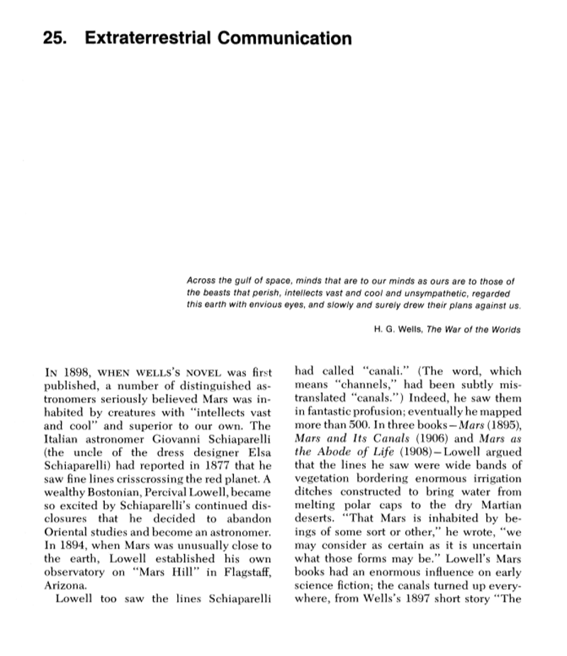
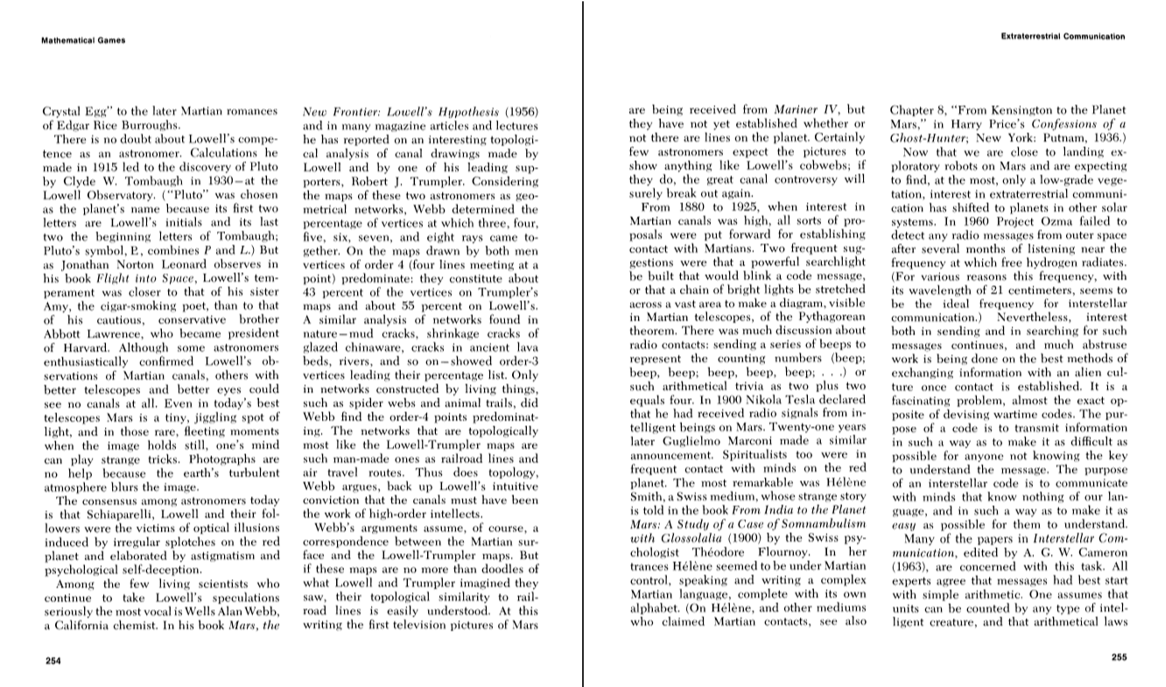
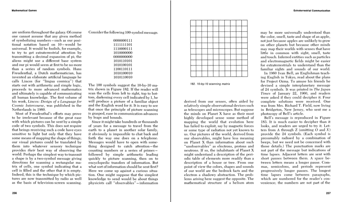
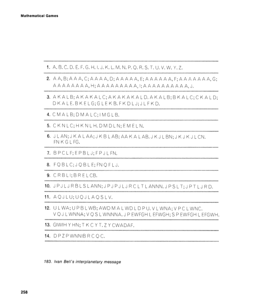
Extraterrestrial Communication Column (Martin Gardner, August 1965)
In 1895, Percival Lowell wrote very, very influential book about Mars (Mars, 1895), inspiring HG Wells and Edgar Rice Burroughs.
When Pluto was found at the Lowell Observatory, P L was chosen to start the planet’s name.
Gardner: “In 1960 Project Ozma failed to detect any radio messages from outer space after several months of listening near the frequency at which free hydrogen radiates. (For various reasons this frequency, with its wavelength of 21 centimeters, seems to be the ideal frequency for interstellar communication.)”
In 1900, Nikola Tesla claimed to have received radio signals from Mars.
Nikola Tesla, “Talking with the Planets,” Collier’s Weekly, February 1901: “I can never forget the first sensations I experienced when it dawned upon me that I had observed something possibly of incalculable consequences to mankind. My first observations positively terrified me, as there was present in them something mysterious, not to say supernatural, and I was alone in my laboratory at night; but at that time the idea of these disturbances being intelligently controlled signals did not yet present itself to me. ... It was some time afterward when the thought flashed upon my mind that the disturbances I had observed might be due to an intelligent control. ... The feeling is constantly growing on me that I had been the first to hear the greeting of one planet to another.”
Nikola Tesla, “Talking with the Planets,” Collier’s Weekly, February 1901: “I can never forget the first sensations I experienced when it dawned upon me that I had observed something possibly of incalculable consequences to mankind. My first observations positively terrified me, as there was present in them something mysterious, not to say supernatural, and I was alone in my laboratory at night; but at that time the idea of these disturbances being intelligently controlled signals did not yet present itself to me. ... It was some time afterward when the thought flashed upon my mind that the disturbances I had observed might be due to an intelligent control. ... The feeling is constantly growing on me that I had been the first to hear the greeting of one planet to another.”
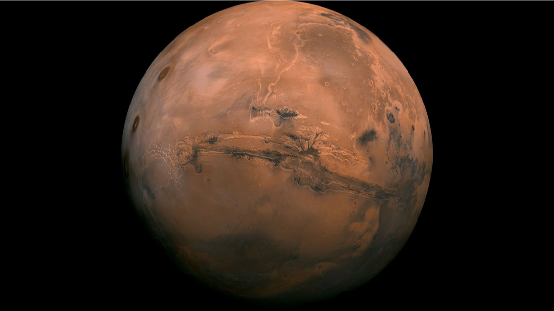
Canals on Mars? Now called the Valles Marineris (1971).
SI Units Standardized (November 16, 2018)
SI Units Standardized (November 16, 2018)
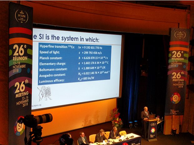
As of 2019, the International System of Units (SI) defines its seven base quantities using fixed values of fundamental physical constants. These constants form the core of our modern metrology.
Base Quantities and Corresponding Constants:
540 THz (≈555 nm) , the most perceived frequency for the human eye. Personally, I’d have gone for 547.533 THz (≈547.533 nm) .
Or a green laser, 532 nm. When they made the color wheel, they should have put green on candela. The luminosity function, V(λ),
was decided in 1924 by the Commission Internationale de l’Éclairage (CIE). Mercury Green = 546.1nm. Chartreuse= 548. Harlequin = 552.
Or a green laser, 532 nm. When they made the color wheel, they should have put green on candela. The luminosity function, V(λ),
was decided in 1924 by the Commission Internationale de l’Éclairage (CIE). Mercury Green = 546.1nm. Chartreuse= 548. Harlequin = 552.
These constants are exact by definition. The SI no longer relies on physical artifacts.
Meter Fight before June 22, 1799
Meter Fight before June 22, 1799
Earth’s gravity varies, but the gravity differential can be measured with a clock and pendulum, as they did at the time.
Several wanted the meter based on the 2-second pendulum: 99.4 cm.
◼
Christiaan Huygens: Made the first practical pendulum clock (1656) and developed the wave theory of light.
◼
Gabriel Mouton: Proposed an early decimal system of measurement based on natural phenomena (1670).
◼
Jean Picard: Performed the first accurate measurement of a degree of longitude in France (1669).
◼
Thomas Jefferson. Second US President. Wanted to redefine the Yard to match the 2-second pendulum.
Others wanted a meridian approach, with 10,000 kilometers from equator to pole.
◼
Antoine Lavoisier: Considered the “Father of Modern Chemistry” for his work on combustion and the conservation of mass.
◼
Joseph-Louis Lagrange: A mathematician and astronomer known for Lagrangian mechanics and celestial mechanics.
◼
Pierre-Simon Laplace: A mathematician and astronomer known for his comprehensive work on celestial mechanics and probability theory.
◼
Jean-Charles de Borda: Developed the “circle of repetition” for precise angular measurements and improved navigation instruments.
◼
Marquis de Condorcet: A prominent Enlightenment philosopher who advocated for human rights and a rational social order.
In the end -- the Meridian won... as such, the distance from the equator to the pole is 10,002 kilometers. They only got 4 digits of accuracy. If they’d gone with the pendulum instead, the distance from the equator to the pole would be 10,062 kilometers. Also, despite difference of gravity, they could have gotten 7 digits of accuracy anywhere in the world.
Defined Constants
Defined Constants
Christiaan Huygens: Made the first practical pendulum clock (1656) and developed the wave theory of light.
Gabriel Mouton: Proposed an early decimal system of measurement based on natural phenomena (1670).
Jean Picard: Performed the first accurate measurement of a degree of longitude in France (1669).
Gabriel Mouton: Proposed an early decimal system of measurement based on natural phenomena (1670).
Jean Picard: Performed the first accurate measurement of a degree of longitude in France (1669).
Derived constants
Derived constants
All of physics can now easily be derived
All of physics can now easily be derived
Drake Equation (1960)
Drake Equation (1960)
Frank Drake led 1960 Project Ozma.
Arecibo Message (1974)
Arecibo Message (1974)
The Arecibo Message was created by Frank Drake , Richard Isaacman, Linda May, astrobiologist James C.G. Walker and Carl Sagan.
The numbers one to ten (white; left to right)
The atomic numbers of the elements hydrogen, carbon, nitrogen, oxygen, and phosphorus, which make up deoxyribonucleic acid (DNA) (purple)
The formulas for the chemical compounds that make up the nucleotides of DNA (green)
H C N O P
1 6 7 8 15
----------
0 0 0 1 1
0 1 1 0 1
0 1 1 0 1
1 0 1 0 1
X X X X X
21 Centimeter Hydrogen Line
21 Centimeter Hydrogen Line
The spin-flip transition of Hydrogen has a wavelength of 21.106114054160(30) cm in a vacuum. On the Pioneer plaque, the line is 21.1 cm.
We can derive Planck’s constant.
AM Radio: About 100 times weaker than an FM radio at 0.000000004 eV (0.004 µeV).
FM Radio: 14 times weaker than the 21 cm line photon at 0.0000004 eV (0.4 µeV).
21 cm Hydrogen Line Photon: This photon has an energy of about 0.000006 eV (6 micro-electronvolts).
CMB Photon: The most energetic CMB photons are about 0.00066 eV (660 µeV).
Visible Light Photon (Red): The light that your eye can see has an energy of about 2 eV. (four hundred million × AM)
Photon Needed to Affect an Atom: To knock the electron completely off of a hydrogen atom (to ionize it) requires 13.6 eV.
X-Ray Photon (Medical): A typical photon used in a medical X-ray has an energy of 50,000 eV.
Our eyes can handle light in the range 10⁻⁶ lux to 1000 lux. The sun is 100,000 lux.
Part of the Pioneer / Voyager plaques
Radio Silence, Please
Radio Silence, Please
Various measures in exact integer relations
Various measures in exact integer relations
Humans have a lot of ways to measure items.
At “A graph of length units that have integer relations with each other”,
I made a graph of distances that have exact integer relations. What is the item at the top?
I made a graph of distances that have exact integer relations. What is the item at the top?
What is the item at the top?
Related: Casimir force : vacuum energy between two parallel uncharged conductive plates. A = area of plates, a = separation.
On Arxiv, Λ is the most popular constant to talk about.
Eratosthenes’ Measurement of the Earth’s Circumference (c. 240 BCE)
Eratosthenes’ Measurement of the Earth’s Circumference (c. 240 BCE)
Eratosthenes measured the circumference of Earth around 240 BC, based on the fact that the Sun appears in the zenith at noon on the summer solstice, in Syene (modern Aswan). At the same time, in Alexandria, the angle of the shadow of a post was slightly more than 7° (you can vary this parameter in this Demonstration), which is roughly 1/50 of the circumference (7/360 ≈ 0.0194444); the distance between the cities is 5000 stadia (an ancient Greek unit, about 185 meters) or about 925 km. The calculation gives 925/.02 ≈ 46250 km, a value very near today’s value of 40000 km, with an error of 16%; an amazing feat for the epoch in which he lived.
Kepler’s Third Law (1619)
Kepler’s Third Law (1619)
Kepler, 1609 (1,2) and 1619 (3)
1. The orbit of a planet is an ellipse with the Sun at one of the two foci.
2. A line segment joining a planet and the Sun sweeps out equal areas during equal intervals of time.
3. The square of a planet’s orbital period is proportional to the cube of the length of the semi-major axis of its orbit.
2. A line segment joining a planet and the Sun sweeps out equal areas during equal intervals of time.
3. The square of a planet’s orbital period is proportional to the cube of the length of the semi-major axis of its orbit.
We can plot this with the solar system:
Newton’s Law of Universal Gravitation (1687)
Newton’s Law of Universal Gravitation (1687)
Key:
Published by Isaac Newton in 1687 in his *Philosophiæ Naturalis Principia Mathematica*, this law described how every mass attracts every other mass with a force proportional to their masses and inversely proportional to the square of the distance between them. It unified earthly physics and celestial motion.
Example: Earth (5.97×10²⁴ kg) and Moon (7.35×10²² kg), distance ≈ 384,400 km
The resulting force is roughly 2×10²⁰ N, which keeps the Moon in orbit.
Cassini and Richer’s Measurement of the Astronomical Unit (1672)
Cassini and Richer’s Measurement of the Astronomical Unit (1672)
Led by the Italian-French astronomer Giovanni Domenico Cassini, this was the first reasonably accurate measurement of the scale of our solar system.
Cassini remained in Paris, France, while his colleague, Jean Richer, was sent on an expedition to Cayenne, French Guiana, in South America. At a prearranged time (when Mars was at its closest point to Earth), both men carefully recorded the position of Mars against the background of distant stars
Because they had a very long baseline (the distance between Paris and Cayenne), they could measure a small but significant parallax angle for Mars. Using trigonometry, this angle allowed them to calculate the distance from Earth to Mars.
At the time, astronomers already knew the relative distances of the planets from the Sun, thanks to Kepler’s Laws of Planetary Motion. They knew, for instance, that Jupiter is about 5.2 times farther from the Sun than Earth is. But they didn’t have a firm number for the actual distance. Cassini’s measurement of the Earth-Mars distance provided the length of the Astronomical Unit (AU)—the distance from the Earth to the Sun. Once the AU was known, the distances to Jupiter, Saturn, and all the other planets could be calculated.
Rømer’s Determination of the Speed of Light (1676)
Rømer’s Determination of the Speed of Light (1676)
Ole Rømer, a Danish astronomer, calculated the speed of light by observing the eclipses of Jupiter’s moon during the years 1668–1674. A discrepancy was observed for the time between the eclipses, increasing when the Earth was moving away from Jupiter and decreasing when the Earth was approaching. In half a year, there are a total of 102 eclipses of Io, giving a maximum delay of 16.5 minutes (shown in the bottom-right plot). Rømer interpreted this as the difference in the times needed for the light to travel between Jupiter and Earth. He obtained a value of 214,000 km/s compared to the current value 299,792 km/s. The diameter of the Earth’s orbit was not accurately known and there was also an error in the measurement of the delay. Nevertheless, it was a first confirmation that the speed of light is finite.
In 1838, Friedrich Bessel was the first to successfully measure the parallax of a star: 61 Cygni. With a heliometer, he measured a parallax of one-third of an arcsecond, placing the star at approximately 10.3 light-years, remarkably close to the modern value. This was the first time humanity measured the distance to a star other than Sol.
Antoine Lavoisier’s Experiments on Conservation of Mass (c. 1770s):
Antoine Lavoisier’s Experiments on Conservation of Mass (c. 1770s):
Lavoisier’s use of sealed containers to weigh reactants and products before and after combustion (of substances like phosphorus and sulfur) was revolutionary. He demonstrated that although matter can change its state, its total mass remains constant. This is a cornerstone of modern chemistry.
In 1794, Joseph Proust carefully measured the ratios by mass of elements in compounds. He showed, for example, that copper carbonate always consisted of the same proportions of copper, carbon, and oxygen, regardless of how it was prepared. This concept of fixed ratios was fundamental to John Dalton’s development of atomic theory.
Schiehallion experiment (1774, measuring Earth’s density)
Cavendish experiment (1797)
Schiehallion experiment (1774, measuring Earth’s density)
Cavendish experiment (1797)
Cavendish experiment (1797)
A pendulum hangs straight downwards in a symmetrical gravitational field. However, if a sufficiently large mass such as a mountain is nearby, its gravitational attraction should pull the pendulum’s plumb-bob slightly out of true (in the sense that it does not point to the centre of mass of the Earth). The change in plumb-line angle against a known object—such as a star—could be carefully measured on opposite sides of the mountain. If the mass of the mountain could be independently established from a determination of its volume and an estimate of the mean density of its rocks, then these values could be extrapolated to provide the mean density of the Earth, and by extension, its mass.
Nevil Maskelyne, Charles Hutton and Reuben Burrow measured Schiehallion, in Scotland, using a 12 in (30 cm) brass quadrant from Cook’s 1769 transit of Venus expedition, a 10 ft (3.0 m) zenith sector, a regulator (precision pendulum clock) for timing the astronomical observations, a theodolite, a Gunter’s chain for surveying the mountain and a pair of barometers for measuring altitude.
Maskelyne calculated a deflection of 20.9 seconds if the mean densities of Schiehallion and the Earth were equal. Since the deflection was about half this, he was able to make a preliminary announcement that the mean density of the Earth was approximately double that of Schiehallion.
Charles Hutton then refined the results, came up with a fairly accurate density measurement, and announced that Earth had a metallic core.
Not long after, Henry Cavendish used a torsion balance made of a six-foot (1.8 m) wooden rod horizontally suspended from a wire, with two 2-inch-diameter (51 mm), 1.61-pound (0.73 kg) lead spheres, one attached to each end. Two massive 12-inch (300 mm), 348-pound (158 kg) lead balls, suspended separately, could be positioned away from or to either side of the smaller balls, 8.85 inches (225 mm) away.
Cavendish found that the Earth’s density was 5.448±0.033 times that of water.
The current accepted value is 5.514 times that of water.
The current accepted value is 5.514 times that of water.
Doppler Shift (1842) and Redshift of Galaxies
Doppler Shift (1842) and Redshift of Galaxies
The effect mentioned by Christian Doppler describes how the observed wavelength of light shifts when a source moves relative to an observer. He described the effect for binary stars. The similar effect for sound came in 1845, from the meteorologist Buys Ballot. For galaxies, redshift reveals recessional velocity and distance.
Fizeau’s Measurement of the Speed of Light (1849)
Fizeau’s Measurement of the Speed of Light (1849)
French physicist Hippolyte Fizeau was the first to successfully measure the speed of light in a terrestrial experiment. His ingenious setup involved a beam of light passing through the teeth of a rapidly rotating cogwheel. The light traveled 8 kilometers (Suresnes to Montmartre) to a mirror and reflected through the same cogwheel.
By increasing the rotation speed of the wheel, Fizeau could find the precise speed at which a tooth would block the returning light. Knowing the distance the light traveled and the rotational speed of the wheel, he calculated a value for the speed of light that was only about 5% off the currently accepted value.
Ludwig Boltzmann, Ideal Gas & Statistical Mechanics (1877)
Ludwig Boltzmann, Ideal Gas & Statistical Mechanics (1877)
In 1877, Boltzmann linked macroscopic gas properties to the statistical behavior of atoms and molecules for the Second Law of Thermodynamics: Entropy never decreases. He gave a probabilistic interpretation of entropy with the equation S=k log W, which relates the entropy (S) of a system to the number of possible microscopic arrangements (W) that correspond to the system’s observed macroscopic state, and k, the Boltzmann constant.
Stefan-Boltzmann Law, Blackbody Radiation (1879)
Stefan-Boltzmann Law, Blackbody Radiation (1879)
The Stefan-Boltzmann law, experimentally discovered by Jožef Stefan in 1879 and later derived from thermodynamic principles by Ludwig Boltzmann, describes the total power radiated from an idealized object known as a “blackbody.”
Max Planck, Law of Blackbody Radiation (1900)
Max Planck, Law of Blackbody Radiation (1900)
This equation gives the spectral radiance of a blackbody at frequency ν and temperature T. It resolved the ultraviolet catastrophe by introducing quantized energy packets.
Planck constant: a photon’s energy is equal to its frequency multiplied by the Planck constant, and the wavelength of a matter wave equals the Planck constant divided by the associated particle momentum.
Boltzmann’s constant: the proportionality factor that relates the average relative thermal energy of particles in a gas with the thermodynamic temperature of the gas.
Example: Plot Planck’s radiation law at 3000 K and 6000 K.
Higher temperature shifts the peak to higher frequencies, avoiding the classical ultraviolet divergence.
Ernest Rutherford and Radiometric Dating (1905)
Ernest Rutherford and Radiometric Dating (1905)
The discovery of radioactivity by Henri Becquerel and the subsequent work by Marie Curie and Bertram Boltwood led to the development of radiometric dating. This allowed scientists for the first time to measure the absolute age of rocks and minerals. It was this measurement that confirmed the Earth was billions of years old, providing the necessary timescale for geological processes and biological evolution.
Ernest Rutherford and Frederick Soddy jointly concluded that radioactivity was caused by a spontaneous transmutation of atomic elements. In radioactive decay, an element breaks down into another, lighter element, releasing alpha, beta, or gamma radiation in the process. They also determined that a particular isotope of a radioactive element decays into another element at a distinctive rate. This rate is given in terms of a “half-life”, or the amount of time it takes half of a mass of that radioactive material to break down into its “decay product”.
Some radioactive materials have short half-lives; some have long half-lives. Uranium and thorium have long half-lives and so persist in Earth’s crust, but radioactive elements with short half-lives have generally disappeared. This suggested that it might be possible to measure the age of Earth by determining the relative proportions of radioactive materials in geological samples. In reality, radioactive elements do not always decay into nonradioactive (“stable”) elements directly, instead, decaying into other radioactive elements that have their own half-lives and so on, until they reach a stable element. These “decay chains”, such as the uranium-radium and thorium series, were known within a few years of the discovery of radioactivity and provided a basis for constructing techniques of radiometric dating.
Some radioactive materials have short half-lives; some have long half-lives. Uranium and thorium have long half-lives and so persist in Earth’s crust, but radioactive elements with short half-lives have generally disappeared. This suggested that it might be possible to measure the age of Earth by determining the relative proportions of radioactive materials in geological samples. In reality, radioactive elements do not always decay into nonradioactive (“stable”) elements directly, instead, decaying into other radioactive elements that have their own half-lives and so on, until they reach a stable element. These “decay chains”, such as the uranium-radium and thorium series, were known within a few years of the discovery of radioactivity and provided a basis for constructing techniques of radiometric dating.
Willard Libby developed carbon dating in the late 1940s at the University of Chicago.
Einstein's Mass–Energy Equivalence (1905)
Einstein's Mass–Energy Equivalence (1905)
First published in 1905 by Albert Einstein in his paper “Does the Inertia of a Body Depend Upon Its Energy Content?”.
Leavitt’s Law (Cepheid Period–Luminosity Relation, 1908)
Leavitt’s Law (Cepheid Period–Luminosity Relation, 1908)
Discovered by Henrietta Swan Leavitt in 1908 and refined in 1912.
She put the pulsation period of Cepheid variable stars and their high and low apparent luminosity on a log plot.
Straight lines indicated a direct relation between period and luminosity, a “standard candle.”
It remains a foundation for measuring distances across the universe.
She put the pulsation period of Cepheid variable stars and their high and low apparent luminosity on a log plot.
Straight lines indicated a direct relation between period and luminosity, a “standard candle.”
It remains a foundation for measuring distances across the universe.
M: Represents the absolute magnitude of the Cepheid.
P: Is the period of pulsation of the Cepheid, typically measured in days.
a and b: Cepheid constants.
P: Is the period of pulsation of the Cepheid, typically measured in days.
a and b: Cepheid constants.
All act as cosmic yardsticks. Measure the period → get M → compare to m → derive distance.
In the spectrum, each of the prominent lines is actually multiple lines:
Johnson–Nyquist noise and Boltzmann constant (1928)
Johnson–Nyquist noise and Boltzmann constant (1928)
Johnson–Nyquist noise can be seen by taking a photo with a sealed digital camera. Instead of getting black, a grainy colored gray results. The warmer the camera, the more the noise. This is why the Webb Space telescope is supercooled.
In 1905, Albert Einstein solved Brownian motion in terms of thermal fluctuations. The following year, in a second paper about Brownian motion, Einstein suggested that the same phenomena could be applied to derive thermally-agitated currents, but did not carry out the calculation as he considered it to be untestable.
In 1927, John B. Johnson working in Bell Labs found noise in communication systems in terms of frequencies. He described his findings to Harry Nyquist, also at Bell Labs, who used principles of thermodynamics and statistical mechanics to explain the results, published in 1928.
Louis Essen and Jack Parry, Microwave Resonance Clock (1955)
Louis Essen and Jack Parry, Microwave Resonance Clock (1955)
The first highly accurate atomic clock, based on the resonant frequency of caesium-133 atoms, was developed by Louis Essen and Jack Parry at the National Physical Laboratory in the UK. By using oscillations of atoms, this clock achieved accuracy far surpassing previous time standards based on the Earth’s rotation. The principle relies on microwaves tuned to the precise frequency that causes electrons in caesium atoms to transition between two specific energy levels. This atomic “pendulum” provided a definition of the second that was both stable and universally reproducible, paving the way for technologies like GPS, global communications, and high-speed data networks.
Meselson-Stahl Experiment (1958):
Meselson-Stahl Experiment (1958):
By using isotopes of nitrogen (“heavy” ¹⁵N and “light” ¹⁴N), Matthew Meselson and Franklin Stahl were able to prove that DNA replication is semi-conservative. They grew bacteria in a ¹⁵N medium, then transferred them to a ¹⁴N medium. By measuring the density of the DNA over subsequent generations using density gradient centrifugation, they showed that each new DNA molecule consisted of one old strand and one new strand.
Raymond Gosling and Rosalind Franklin, Photo 51 (DNA, 1953)
Raymond Gosling and Rosalind Franklin, Photo 51 (DNA, 1953)
Diffraction photograph of DNA.
Gosling showed it to Maurice Wilkins,
who showed it to James Watson,
who showed it to Francis Crick,
who had written about what the diffraction pattern of a helix would be.
Gosling showed it to Maurice Wilkins,
who showed it to James Watson,
who showed it to Francis Crick,
who had written about what the diffraction pattern of a helix would be.
Cosmic Microwave Background ( Arno Allan Penzias and Robert Woodrow Wilson, 1965)
Cosmic Microwave Background ( Arno Allan Penzias and Robert Woodrow Wilson, 1965)
Microwave radiation that fills all space in the observable universe.
Universe Lengths at various scales
Universe Lengths at various scales
Why do we see 400–700 nm ?
Why do we see 400–700 nm ?
Because dangerous photons out of this range are mostly absorbed by the atmosphere.
Isn’t that convenient?
Isn’t that convenient?
Astronomers use high-altitude, balloon, or satellite instruments to observe in UV and IR precisely because Earth blocks those bands.
Many of the strongest spectral lines are in the range:
Numbers and Elements -- What can we expect?
Numbers and Elements -- What can we expect?
Communicating with aliens on other worlds, we should assume that they know a few things.
1. Numbers – A concept of discrete counting: 1, 2, 3, etc. Zero. Positional notation. Prime numbers. Fractions and ratios.
2. Geometry – Recognition of lines, angles, circles, triangles, right triangles. Spatial awareness. Dimension, symmetry and coordinate systems.
3. Time perception – Experience of periodicity (pulses, cycles, decay), duration and intervals.
4. Physical constants – Familiarity with constants like the speed of light, Planck’s constant or the fine-structure constant.
5. Chemical elements – Knowledge of atoms, hydrogen, helium, carbon, oxygen and nitrogen. The Periodic table and chemistry.
6. Electromagnetic spectrum – Use of radio, microwave, or optical signals for detection or communication.
7. Measurement and comparison – Perhaps based on their own cultures.
8. Language, symbol systems and logic structures – Use of internal or external notation to store, compare, or manipulate data.
9. Itemized lists – Grouping and sequencing of ideas or objects, likely structured hierarchically or sequentially.
Extragalactic Distance Ladder
Extragalactic Distance Ladder
Type Ia supernova peak luminosity:
Type Ia supernova peak luminosity:
The typical visual absolute magnitude of Type Ia supernovae is Mv = −19.3 (about 5 billion times brighter than the Sun), with little variation. The similarity in the absolute luminosity profiles of nearly all known Type Ia supernovae has led to their use as a secondary standard candle in extragalactic astronomy.
(wikipedia) The Type Ia category of supernova produces a fairly consistent peak luminosity because of the fixed critical mass at which a white dwarf will explode. Their consistent peak luminosity allows these explosions to be used as standard candles to measure the distance to their host galaxies: the visual magnitude of a type Ia supernova, as observed from Earth, indicates its distance from Earth.
Even when dust or other material in the area of the supernova disrupts the observation, the luminosity plot predictable enough that the observation can be mapped to it.
Chirp Mass Distribution (Standard Siren)
Chirp Mass Distribution (Standard Siren)
In astrophysics, the chirp mass of a compact binary system determines the leading-order orbital evolution of the system as a result of energy loss from emitting gravitational waves. Because the gravitational wave frequency is determined by orbital frequency, the chirp mass also determines the frequency evolution of the gravitational wave signal emitted during a binary’s inspiral phase. In gravitational wave data analysis, it is easier to measure the chirp mass than the two component masses alone.
Heidelberg Institute for Theoretical Studies (HITS)
Baryon Acoustic Oscillations
Baryon Acoustic Oscillations
Fluctuations in the density of matter in the universe, caused by acoustic density waves in the primordial plasma of the early universe.
1. The Ripple: In the hot, dense early universe, sound waves rippled outward from any spot that was slightly denser than average, like dropping a pebble in a pond.
2. The Freeze: After 380,000 years, the universe suddenly became transparent. The pressure driving the sound waves vanished, and the ripples froze instantly in place.
3. The Ruler: These frozen ripples created a preferred distance for where galaxies would later form. Today, we see this as a slight tendency for galaxies to be separated by about 490 million light-years.
What happens with randomly placed points with a BAO type spike? Start with points on a sphere:
Trying out these values, we get patterns similar to galaxy distributions:
How do we communicate Stellar Mass with an Alien?
How do we communicate Stellar Mass with an Alien?
Let W = .55 M☉, the Stellar Remnant Constant.
1W peak for the mass distribution of He I lines white dwarfs (HB).
2W lightest neutron star, heaviest observed white dwarfs.
3W peak for the mass distribution of neutron stars.
4W Tolman–Oppenheimer–Volkoff limit. Beyond 2.2 M☉, you get a black hole.
1W peak for the mass distribution of He I lines white dwarfs (HB).
2W lightest neutron star, heaviest observed white dwarfs.
3W peak for the mass distribution of neutron stars.
4W Tolman–Oppenheimer–Volkoff limit. Beyond 2.2 M☉, you get a black hole.
What else can be used for Mass?
What else can be used for Mass?
Proton mass: ~ 1.6726e-27 kg | ~ 938.27 MeV/c^2
Neutron mass: ~ 1.6750e-27 kg | ~ 939.57 MeV/c^2
Electron mass: ~ 9.1094e-31 kg | ~ 0.511 MeV/c^2
Planck mass: ~ 2.1765e-08 kg | ~ 1.22e+22 MeV/c^2
H atom mass: ~ 1.6735e-27 kg | ~ 938.78 MeV/c^2
Carbon-12 mass: exactly 12 u | ~ 11177.9 MeV/c^2
Top quark mass: ~ 3.1e-25 kg | ~ 174,000 MeV/c^2
Neutron mass: ~ 1.6750e-27 kg | ~ 939.57 MeV/c^2
Electron mass: ~ 9.1094e-31 kg | ~ 0.511 MeV/c^2
Planck mass: ~ 2.1765e-08 kg | ~ 1.22e+22 MeV/c^2
H atom mass: ~ 1.6735e-27 kg | ~ 938.78 MeV/c^2
Carbon-12 mass: exactly 12 u | ~ 11177.9 MeV/c^2
Top quark mass: ~ 3.1e-25 kg | ~ 174,000 MeV/c^2
MegaElectrovolt/c^2 : 1.78266192e-30 kg
iron-56 binding energy = 492.253892 MeV (nuclear reactions unfavorable)
iron-56 binding energy = 492.253892 MeV (nuclear reactions unfavorable)
Dangerous spheres: sizes to aim for:
~0.012 M☉ - The Deuterium Burning Limit: Brown Dwarf.
~0.075 M☉ - The Hydrogen Burning Limit: Red Dwarf helium white dwarfs
~0.5 - 2.0 M☉ - Helium Flash Stars red giants carbon-oxygen white dwarfs.
~2.0 - 8.0 M☉ - Helium Fusion Stars red giants oxygen-neon-magnesium white dwarfs.
~8.0 - 20 M☉ - Supernova Neutron star
~20+ M☉ - Black Hole Progenitors
~0.075 M☉ - The Hydrogen Burning Limit: Red Dwarf helium white dwarfs
~0.5 - 2.0 M☉ - Helium Flash Stars red giants carbon-oxygen white dwarfs.
~2.0 - 8.0 M☉ - Helium Fusion Stars red giants oxygen-neon-magnesium white dwarfs.
~8.0 - 20 M☉ - Supernova Neutron star
~20+ M☉ - Black Hole Progenitors
Only Bright And Fiery Globes Know More Luminosity Than You.
Only Bright And Fiery Globes Know More Luminosity Than You.
Stellar classifications immediately give many standards. I disliked the mnemonic so I made a better one.
Class | Star Name | Temp (K) | Mass (Solar) | Luminosity (Solar) | Distance (ly) | Note
------|-----------------------|------------|--------------|--------------------|---------------|----------------------------------------------------
O | Zeta Puppis | ~40,000 K | ~25 | ~440,000 | ~1,090 | Extremely hot and luminous blue supergiant
B | Rigel | ~12,100 K | ~21 | ~120,000 | ~860 | Bright blue-white supergiant in Orion
A | Sirius | ~9,940 K | ~2.06 | ~25.4 | 8.6 | Brightest star in Earth’s night sky
F | Procyon | ~6,530 K | ~1.5 | ~6.9 | 11.5 | Appears yellowish-white to the naked eye
G | The Sun (Sol) | 5,778 K | 1.0 | 1.0 | 0.0000158 | Our own star, the definition of Solar units
K | Epsilon Eridani | ~5,084 K | ~0.82 | ~0.34 | 10.5 | Nearby orange dwarf with a debris disk
M | Proxima Centauri | ~3,042 K | ~0.12 | ~0.0017 | 4.2 | Closest known star to the Sun, hosts planets
L | 2MASS J0523-1403 | ~2,075 K | ~0.04 | ~0.000126 | ~40 | One of the smallest known true stars
T | Epsilon Indi Ba | ~1,300 K | ~0.045 | ~0.00003 | ~12 | Methane brown dwarf, part of a nearby system
Y | WISE 0855−0714 | ~250 K | ~0.003 | ~0.0000003 | ~7.4 | One of the coldest brown dwarfs, colder than Earth
Biological Size Limits
Biological Size Limits
In mammals, blood cells aren’t nucleated, which allows more hemoglobin and thus a greater oxygen capacity. It also conveys a greater ability to handle dehydration, since RBC can vary 50% in size. An extreme example is camels, where RBC can vary 240% in size.
For nucleated cells, the genome and cell machinery must be stored. This sets a minimal nucleated cell size of about 10 micrometers (μm), approximately the thickness of plastic wrap. As a cell grows larger, diffusion of resources and wastes becomes difficult, and the metabolic burden increases. There are only so many mRNA instructions a nucleus can send out. Thus, for all cells supporting a larger structure, there are practical upper and lower limits on size. Single-celled organisms and specialized cells can violate these boundaries, but only with specific adaptations.
Biological Time
Biological Time
Cells operate on many timescales, but their fastest and most universal processes unfold at the microsecond level. This is the domain of electrical responses, ion motion, and critical first steps in signaling. One of the fastest is Ion channel gating at ~1 millisecond. Most action in a cell happens in terms of milliseconds.
1× | Electrical | Ion channel gating (Na⁺, K⁺, Ca²⁺)
1× | Electrical | Fast Na⁺ channel opening
1× | Electrical | Action potential rise time (Na⁺ influx)
1× | Electrical | AMPA receptor channel activation
2× | Electrical | Voltage sensor movement (S4 domain)
2× | Metabolic | ATP hydrolysis catalytic turnover (typical ATPase)
2× | Metabolic | Glucose transporter (GLUT1) conformational shift
3× | Electrical | Action potential rise (continued Na⁺ influx)
3× | Metabolic | Lactate dehydrogenase catalytic turnover
4× | Electrical | Membrane charging time (typical neuron RC constant)
5× | Transport | Synaptic cleft neurotransmitter diffusion
5× | Metabolic | Glycolytic enzyme turnover (e.g., Hexokinase)
5× | Structural | Lipid flip-flop across bilayer (enzymatic)
6× | Mechanical | Kinesin motor single step (~8 nm)
7× | Mechanical | Myosin power stroke in muscle
8× | Mechanical | ATP-driven chaperone conformational cycle (e.g., Hsp70)
9× | Mechanical | Rotary step of bacterial flagellum motor
10× | Electrical | AMPA receptor activation (duplicate phrasing, may omit)
10× | Mechanical | SNARE complex zippering and vesicle fusion
10× | Mechanical | Kinesin motor single step (alt phrasing, see 6×)
10× | Metabolic | ATP synthase H⁺ rotation step
15× | Metabolic | GTP hydrolysis by Ras
18× | Mechanical | Clathrin triskelion recruitment step
20× | Electrical | EPSP/IPSP rise to peak
20× | Metabolic | Krebs cycle enzyme turnover (e.g., Citrate Synthase)
25× | Electrical | Chloride channel gating (e.g., CFTR)
30× | Synaptic | Vesicle fusion and release
35× | Sensory | Rod photoreceptor cGMP-gated channel closure
40× | Sensory | Olfactory receptor signal initiation cascade
45× | Mechanical | Intermediate filament unit annealing
50× | Signaling | GPCR ligand binding
60× | Mechanical | Dynein stepping motion
75× | Signaling | Calcium-dependent calmodulin binding onset
80× | Mechanical | Dynein motor stepping motion (merged entry)
90× | Mechanical | Basal cilia beat initiation
100× | Signaling | G-protein activation (GDP-GTP exchange)
100× | Transport | Vesicle clearance from synaptic cleft
120× | Mechanical | Tight junction sealing wave (per protein unit)
150× | Mechanical | Tubulin dimer addition to growing microtubule
180× | Signaling | Rapid phosphorylation cascade (e.g., JNK/MAPK first tier)
200× | Signaling | Second messenger spike onset (cAMP, IP₃)
220× | Transport | Nuclear pore complex passive diffusion (<40 kDa proteins)
250× | Metabolic | tRNA charging by aminoacyl-tRNA synthetase
300× | Signaling | Calcium wave nucleation and propagation
300× | Mechanical | Golgi vesicle budding event
400× | Mechanical | Microvilli probing (immune cell)
400× | Structural | ER shape modulation cycle
480× | Mechanical | Primary cilium bending in response to flow
500× | Structural | Actin filament nucleation burst
500× | Signaling | GPCR signaling cascade begins
600× | Mechanical | Focal adhesion initial formation (alt phrasing)
700× | Signaling | Transient PKC anchoring at membrane
800× | Structural | Initial formation of focal adhesions
850× | Transport | V-ATPase proton pumping cycle (per rotation)
1000× | Transport | Mitochondrial Ca²⁺ uptake via the uniporter
1000× | Mechanical | Mitochondrial fission initiation
1 s | Structural | Cytoskeletal patch remodeling
1 s | Transport | Mitochondrial Ca²⁺ uptake via the uniporter
1 s | Respiratory | Oxygen loading/unloading by red blood cells in capillaries
1.2 s | Metabolic | Enzyme complex reconfiguration (e.g., PDH reset)
2 s | Mechanical | Lysosome migration to periphery
3 s | Signaling | Ca²⁺-dependent transcription factor activation (e.g., NFAT nuclear entry)
5 s | Transport | mRNA localization within cytoplasm
6 s | Metabolic | Full glycolytic pathway (glucose to pyruvate)
10 s | Metabolic | One full turn of the Krebs cycle
10 s | Structural | Actin treadmilling cycle
15 s | Mechanical | Large cargo vesicle transport across cell
20 s | Signaling | Receptor endocytosis and early endosome formation
30 s | Structural | Microtubule network reorganization
60 s | Transcriptional | RNA polymerase II initiation and promoter escape
120 s | Transcriptional | Primary transcript splicing
180 s | Structural | Golgi apparatus recovery after insult
300 s | Polarity | Full cell polarity reorientation
600 s | DNA Repair | Damage recognition and repair dwell
1000 s | Epigenetic | Chromatin remodeling and histone modification cascade
1800 s | Developmental | Cell fate reprogramming (e.g., Yamanaka response)
Triple Point, Critical Point and Superconductance
Triple Point, Critical Point and Superconductance
In thermodynamics, the triple point of a substance is the temperature and pressure at which the three phases (gas, liquid, and solid) of that substance coexist in thermodynamic equilibrium. The critical point is the end point of the pressure–temperature curve that designates conditions under which a liquid and its vapor can coexist.
Before 2019, the triple point of water was used to define the kelvin.
Some triple points and critical points.
Temperature where electrical resistance vanishes and magnetic fields are expelled.
The current leader is Lanthanum decahydride, with a superconducting transition temperature
of 250 K (−23 °C; −10 °F), but it is only stable at a pressure of 150 gigapascals.
of 250 K (−23 °C; −10 °F), but it is only stable at a pressure of 150 gigapascals.
The Planck Energy Unit, which I call ♇.
The Planck Energy Unit, which I call ♇.
At the start, I showed Martin Gardner’s 1965 column, where he mention Percival Lowell, who had an observatory which discovered Pluto. Clyde Tombaugh replied to the column, and Martin Gardner responded. I consider ♇ to be an excellent monetary unit.
The buying power of 1 ♇ has been incredibly stable for over a hundred years.
Michael Trott (1959-2025)
Michael Trott (1959-2025)
At the State Department, to collect the 2005 Carl Sagan Award for Public Appreciation of Science, for work on Numb3rs.
CITE THIS NOTEBOOK
CITE THIS NOTEBOOK
Mathematical Games 30: Measuring the Universe
by Ed Pegg
Wolfram Community, STAFF PICKS, June 26, 2025
https://community.wolfram.com/groups/-/m/t/3486408
by Ed Pegg
Wolfram Community, STAFF PICKS, June 26, 2025
https://community.wolfram.com/groups/-/m/t/3486408