Quadratic Forms
Quadratic Forms
In this notebook, we'll see level curves of some quadratic forms and how the shape is changing depending on some coefficients.
■
First, let's see how it is changing depending on the level curve value.
The animation below, gives two examples that have different graphs so that we can see the effect in these two different cases.
Notice that the range starts from 0. Also, depending on the middle term, we have an ellipse or a hyperbola.
The animation below, gives two examples that have different graphs so that we can see the effect in these two different cases.
Notice that the range starts from 0. Also, depending on the middle term, we have an ellipse or a hyperbola.
In[]:=
Animate[{ContourPlot[4x^2+5x*y+4y^2==a,{x,-3,3},{y,-3,3},AxesTrue],ContourPlot[4x^2+10x*y+4y^2==a,{x,-3,3},{y,-3,3},AxesTrue]},{a,0,15},AnimationRunningFalse,DisplayAllStepsTrue]
Out[]=
■
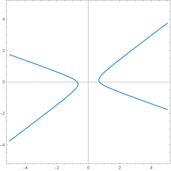
In the previous work, level curves are different as a result of different middle terms. Let's explore how the shape is changing depending on the coefficient in the middle.
Following work also includes the symmetric matrix corresponding to the quadratic form and its eigenvalues and eigenvectors.
Following work also includes the symmetric matrix corresponding to the quadratic form and its eigenvalues and eigenvectors.
◼
Questions:
What is the relationship between the shape and eigenvalues of A?
What is the relationship between the shape and eigenvectors of A?
What is the relationship between the shape and eigenvalues of A?
What is the relationship between the shape and eigenvectors of A?
In[]:=
Manipulate[ContourPlot[4x^2+ax*y+4y^2==2,{x,-5,5},{y,-5,5},AxesTrue],{{a,-15,"a-value"},-15,15,1},Style["Matrix",12,Bold],Dynamic[{{4,a/2},{a/2,4}}//MatrixForm],Delimiter,Style["First Eigenvalue-Eigenvector",12,Bold],Dynamic[Eigensystem[{{4,a/2},{a/2,4}}][[1]][[1]]],Dynamic[Eigensystem[{{4,a/2},{a/2,4}}][[2]][[1]]//MatrixForm],Style["Second Eigenvalue-Eigenvector",12,Bold],Dynamic[Eigensystem[{{4,a/2},{a/2,4}}][[1]][[2]]],Dynamic[Eigensystem[{{4,a/2},{a/2,4}}][[2]][[2]]//MatrixForm],ControlPlacementLeft]
Out[]=

■
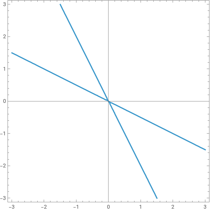
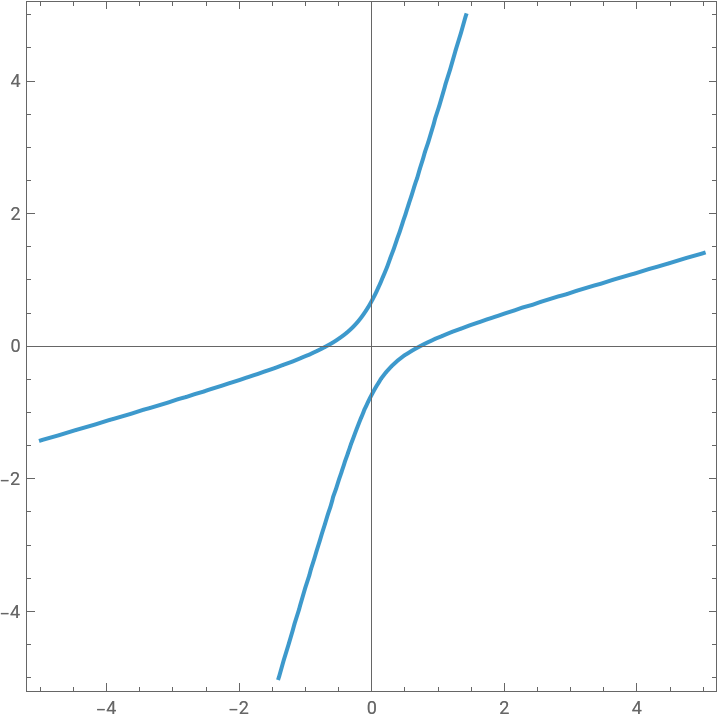
Now, let's keep the first two coefficients fixed and vary the coefficient of y^2 term. We can again observe the change in the shape depending on the eigenvalues and eigenvectors.
Now, let's keep the first two coefficients fixed and vary the coefficient of y^2 term. We can again observe the change in the shape depending on the eigenvalues and eigenvectors.
In[]:=
Manipulate[ContourPlot[4x^2+6x*y+ay^2==2,{x,-5,5},{y,-5,5},AxesTrue],{{a,-15,"a-value"},-15,15,1},Style["Matrix",12,Bold],Dynamic[{{4,3},{3,a}}//MatrixForm],Delimiter,Style["Eigenvalues",12,Bold],Dynamic[N[Eigensystem[{{4,3},{3,a}}][[1]][[1]]]],Dynamic[N[Eigensystem[{{4,3},{3,a}}][[1]][[2]]]],Delimiter,Style["Corresponding Eigenvectors",12,Bold],Dynamic[N[Eigensystem[{{4,3},{3,a}}][[2]][[1]]]//MatrixForm],Dynamic[N[Eigensystem[{{4,3},{3,a}}][[2]][[2]]]//MatrixForm],ControlPlacementLeft]
Out[]=