On the 14 September 2020 episode of , Tom and Ray posed the following puzzler. (A transcript, available , is well worth reading). I like this puzzler because the proposed answer, though incorrect, has a certain playful appeal. It also gives an excuse to play with Integrate, Region, and ProbabilityDistribution.
The fuel tank of a truck has the shape of a cylinder on it’s side, with a filler hole on top. When the tank is half full of fuel, a broomstick inserted through the filler opening will be marked at half the tanks’s diameter. Where is the stick marked when the tank is 1/4 full?
The proposed answer involves a circular cardboard disk, as typically found under a pizza. The circular disk is sliced precisely in half, and the point where the half-disk balances on a pencil point is found. This point is said to indicate the fuel level when the tank is 1/4 full.
This figure will help clarify ideas and notation.
Plot[{1-Sqrt[1-],Callout[If[1-Sqrt[1-]<0.45,0.45,None],"Fuel Level h",Scaled[0.2]]},{x,-1,1},Epilog{Text["Area Beneath\nChord (ABC)",{0.3,0.3}]},Filling{1{2}},ImageSize400,FrameTrue,FrameLabel{x,Rotate[y,-π/2]},PlotLabel"Cross section of fuel in a cylindrical tank (partial view)\n\t Blue curve is y=1-Sqrt[1-x^2]"]
2
x
2
x
Out[]=
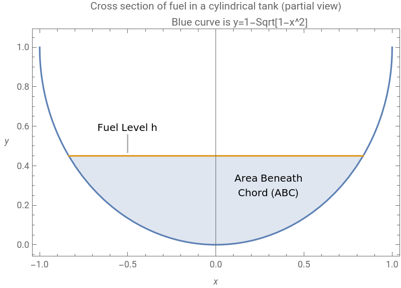
The figure represents half the fuel tank along with some fuel; clearly, a stick inserted vertically through the filler cap will be wetted to a level . The shaded two-dimensional area serves as a proxy for fuel volume, and we’ll attempt to reduce verbiage by referring to it as the Area Beneath Chord, or ABC. Our unit circle has total area , and so when , when , etc. The challenge is to find that makes .
h
π=π
2
r
ABC=π
h=2
ABC=π/2
h=1
h
ABC=π/4
The point along on which a cardboard semicircle will balance is proposed as the correct value of . This is plausible: after all, a cardboard shape balanced on a point has “equal stuff” all around, right? Unfortunately, what’s equal is the torques, and not necessarily the masses (though this approach would work for a rectangular tank). A remedy is possible with a balance scale: the cardboard can be sliced along a candidate fuel level, and the problem is solved when the two pieces put the scale in equilibrium. The only disadvantage is that trial and error, and perhaps a lot of cardboard, is required.
x=0
h
Fortunately, cardboard-free solutions are possible.
A Solution using Integrate
A Solution using Integrate
Our fuel tank is represented by a unit circle centered at (0,1). We’ll need as a function of for Integrate, and again below in ProbabilityDistribution.
x
y
Solve[+1,x]
2
x
2
(y-1)
Out[]=
x-
2y-
,x2
y
2y-
2
y
The amount of fuel in the tank is related to as follows.
h
Clear[abc];abc=Integrate[1,{y,0,h},{x,-Sqrt[2y-],Sqrt[2y-]},Assumptions0<h<2]
2
y
2
y
Out[]=
-
(2-h)h
+-(-2+h)
+2ArcSin3
h
h
2
This plot shows how ABC goes from 0 to π as goes from 0 to 2.
h
Plot[abc,{h,0,2},FrameTrue,FrameLabel{"h","ABC"},PlotLabel"Area Beneath Chord as a function of h"]
Out[]=
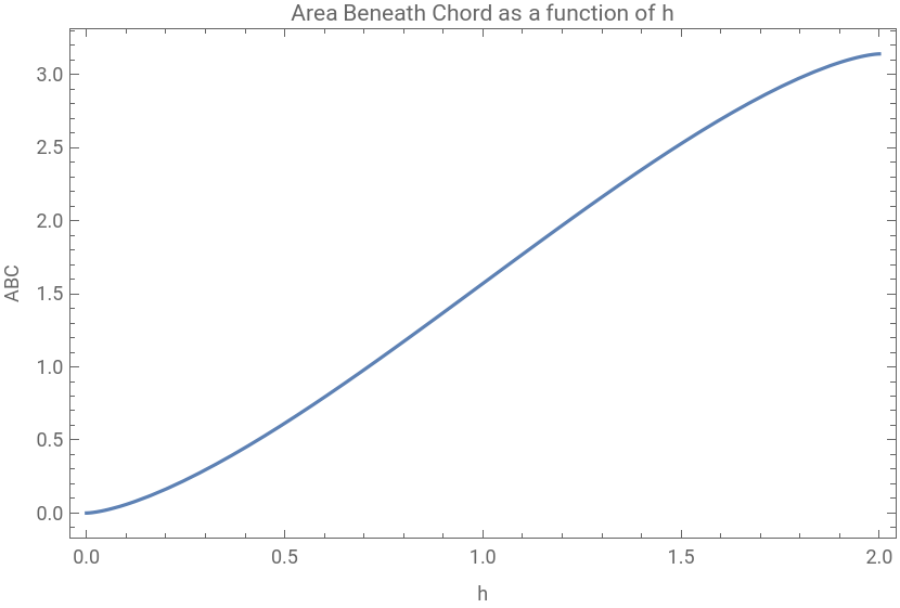
It turns out that Solve can express as a Root.
h
Solve[abcπ/4,h,Reals];{%,N@%}//Flatten
Out[]=
h,h0.596027

This result passes a basic dummy check.
Column[{π/4,abc/.First[%7]}//N[#,24]&]
Out[]=
0.785398163397448309615661 |
0.785398163397448309615661 |
The point about which the semicircle of cardboard will balance is slightly less than .
p
h
EqualIntegrate(p-y)
2y-
,{y,0,p},Assumptions0<p<1,Integrate(y-p)2
y
2y-
,{y,p,1},Assumptions0<p<1;Solve[%,p];{%,N@%}//Flatten2
y
Out[]=
p,p0.575587
-4+3π
3π
A Solution using Region, Area, and RegionCentroid
A Solution using Region, Area, and RegionCentroid
These results can be checked with RegionCentroid and RegionMeasure.
As expected, RegionCentroid gives the we found above.
p
{Region[#],RegionCentroid[#]}&@ImplicitRegion[+<1&&y<1,{x,y}]
2
x
2
(y-1)
Out[]=
,0,

-4+3π
3π
I’ve had no luck finding using Area or RegionMeasure with Solve, NSolve, or FindRoot. It seems that Solve cannot “see inside” ImplicitRegion, though a little voice inside my head says I may be overlooking something…
h
Solve[RegionMeasure[ImplicitRegion[+<1&&y<h,{x,y}]]π4,h,Reals]
2
x
2
(-1+y)
Out[]=
{}
The following is a bit clunky, but at least it gives an close to what we found above.
h
areaInterpolation=Interpolation[Table[{h,RegionMeasure[ImplicitRegion[+<1&&y<h,{x,y}]]},{h,0,1,0.01}]];FindRoot[areaInterpolation[h]π/4,{h,0.5}];{%,(h/.First[%7])-(h/.%)}//Flatten
2
x
2
(y-1)
Out[]=
{h0.596027,-1.46245×}
-9
10
A Solution using Mean and Median
A Solution using Mean and Median
Mean and Median give the and found above, and do so with the most concise, and perhaps most transparent, code. Here mass is represented as probability, with mean and median summarizing the PDF as discussed above.
h
p
ProbabilityDistribution"PDF",
2y-
,{y,0,1},Method"Normalize";{Mean[%],Median[%]}2
y
Out[]=
,
-4+3π
3π
A Crazy Thought
A Crazy Thought
It’s been said that every problem-solving mistake is either an error, or a blunder [3]. Though most would--with some justification--disagree, I argue that the mistake discussed here is only an error, and a mild one at that. Any solution to any problem has many facets, and being correct (or not) is sometimes the least interesting of a suggested solution's many personality characteristics.
References
References
[3] Householder, Alston S., Principles of Numerical Analysis. Dover Publications, 1981.