Abstract: Monte Carlo Simulations are a popular method for the evaluation of investment projects containing stochastic components, such as (but not limited to) the uncertain future development of cost, prices or interest rates. The Wolfram Language provides a handy, computationally robust foundation for the modeling and analysis of random paths generated by various parametric random processes and/or stochastic differential equations. While some of those processes have apparently been implemented in a reasonably efficient manner, less commonly used ones - such as the Cox-Ingersoll-Ross-Process - aren’t calculating as fast as the (notoriously impatient) author would expect them to calculate.
In this short Notebook we will - from the perspective of the user of an Apple MacBook Pro with an M3 processor - have a look at the timing of the generation of one million random paths of the Cox-Ingersoll-Ross (CIR) process using
(a) the Wolfram Language’s built-in RandomFunction (reference),
(b) a naive implementation using Table, FoldList and Compile-to-C (about 150 times faster),
(c) an approach using OpenCLLink (about 1.000 times faster),
(d) a C++ implementation called via the Foreign Function Interface (6.000 times faster), and
(e) an Objective-C / Metal implementation, also called via the Foreign Function Interface (8.000 times faster).
We see, that - aided by very efficient and well-thought out interfaces built into the Wolfram Language and its ability to allocate and share raw memory - overcoming performance issues with certain built-in functionality is possible in a relatively pain- and frictionless manner.
We also see, that although the Wolfram Language doesn’t yet provide a direct interface to Apple’s Metal shader API (analogous to the very useful CudaLink and OpenCLLink packages), we can easily and efficiently invoke GPU computations on Apple Silicon via Mathematica’s Foreign Function Interface, using Objective-C as a bridge.
From a mathematical point of view, we learn, that common discretization techniques for Stochastic Differential Equations may fail to yield acceptably accurate results when large discretization step sizes are chosen.
1. Hardware and Software Specs
The present Notebook was developed and tested on a system with the following specifications:
Model Name: Apple MacBook Pro Chip: Apple M3 Max Total Number of Cores: 16 (12 Performance, 4 Efficiency) Memory: 128 GB System Version: macOS 14.3 (Sonoma, 23D56) Mathematica Version: 14.1.0.0
2. The Cox-Ingersoll-Ross Process
2.1. Definition
2.1. Definition
The Cox-Ingersoll-Ross (CIR) model is a mean-reverting one-factor-model commonly applied to describe the evolution of interest rates over time. It describes a stochastic process defined by the following stochastic differential equation:
dx(t)θ(μ-x(t))dt+σ·
x(t)
dw
t
(
1
)Here, is a Wiener-process, μ is the long-term mean, θ is the speed of adjustment towards the mean (rate of mean-reversal) and x(0) would be the initial condition (which may or may not be different from μ).
w
t
2.2. Wolfram Implementation
2.2. Wolfram Implementation
In the Wolfram Language, the CIR-Process is conveniently implemented as CoxIngersollRossProcess[μ, σ, θ, x0].
n random paths can be generated from that process by RandomFunction[process,{t1,t2,dt},n].
Mean and Standard Deviation
Mean and Standard Deviation
The theoretical mean of the slice distribution of a CIR - process at time t is
x
0
-θt
e
-θt
e
(
2
)In[]:=
fCIRMean=x0*Exp[-t*θ]+μ*(1-Exp[-t*θ]);
The theoretical standard deviation of the slice distribution of a CIR-process at time t is:
x
0
2
σ
2θ
-θt
e
-θt
e
2
σ
2θ
2
(1-)
-θt
e
(
3
)In[]:=
fCIRStdDev=Sqrt[x0*σ^2/(2*θ)*Exp[-θ*t]*(1-Exp[-θ*t])+μ*σ^2/(2*θ)*(1-Exp[-θ*t])^2];
Checking Wolfram Implementation
Checking Wolfram Implementation
We are now having a look at the CoxIngersollRoss process as implemented in the Wolfram language.
In[]:=
Block[{μ=1.0,σ=0.25,θ=0.65,x0=1.0,t=25,paths,slice25},cirpForCheck=CoxIngersollRossProcess[1.0,0.25,0.65,1.0];paths=RandomFunction[cirpForCheck,{0,25,1},10000];slice25=paths["ValueList"][[All,26]];TableForm[{{"Mean:",Mean@paths,fCIRMean},{"StandardDeviation:",StandardDeviation@paths,fCIRStdDev}},TableHeadings->{None,{"","Wolfram Random Function","Theoretical"}}]]
Out[]//TableForm=
Wolfram Random Function | Theoretical | |
Mean: | 0.999785 | 1. |
StandardDeviation: | 0.213848 | 0.219264 |
As can be seen from the above results, the mean and standard distribution of the slice of our exemplary CIR process closely match the theoretical values. Thus Wolfram’s implementation seems to be correct. However it appears to be relatively slow, which warrants further investigation and experiments.
2.2. Example
2.2. Example
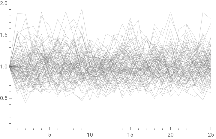
We are - as the motivation to study the present matter comes from a practical example the author had to work on - assuming μ = 1.0, σ = 0.25, θ = 0.65 and x(0) = 1.0.
The Wolfram Language allows us to conveniently create and visualize any number n of random paths of length m for this process with the following code:
The Wolfram Language allows us to conveniently create and visualize any number n of random paths of length m for this process with the following code:
In[]:=
Module[{μ=1.0,σ=0.25,θ=0.65,x0=1.0,n=100,m=25,model,randomPaths},model=CoxIngersollRossProcess[μ,σ,θ,x0];randomPaths=RandomFunction[model,{0,m,1},n];ListLinePlot[randomPaths,PlotStyle->{{Gray,Thin}}]]
Out[]=
The implementation of the CIR-Process in the Wolfram allows for symbolical as well as numerical evaluation, and the result of RandomFunction provides the following convenient properties:
Out[]=
Components | DateList | DatePath | DatePaths |
Dates | FirstDates | FirstTimes | FirstValues |
LastDates | LastTimes | LastValues | Part |
Path | PathComponent | PathComponents | PathCount |
PathDates | PathFunction | PathFunctions | PathLength |
PathLengths | Paths | PathTimes | SliceData |
SliceDistribution | TimeList | Times | ValueDimensions |
ValueList | Values | | |
For the purpose of our Monte Carlo simulation, we shall be interested only in “ValueList”, though.
3. Benchmarking the CIR Implementation
Let us assume now, that we require 1 Million independent random CIR-paths of length 26 (indexed from 0 to 25) for our Monte Carlo Simulation, and time, how long it takes to generate them.
3.1. CIR - Built In Implementation
3.1. CIR - Built In Implementation
We shall call the below timing function for values of n ranging from 1000 to 1.000.000 (stepping in multiples of 10) and table the resulting execution times. N.b.: We deliberately avoid outputting the results of the path generation itself, in order to avoid distortion of measurements by I/O and formatting operations.
In[]:=
cirBuiltinTiming[n_]:=Module[{μ=1.0,σ=0.25,θ=0.65,x0=1.0,m=25,model,randomPaths},model=CoxIngersollRossProcess[μ,σ,θ,x0];randomPaths=RandomFunction[model,{0,m,1},n];]//AbsoluteTiming;
Helper Function for Tabling Timing of Path Generation
Helper Function for Tabling Timing of Path Generation
In[]:=
timingTable[functionOfN_]:=TableForm[Table[{10^exp,functionOfN[10^exp][[1]]},{exp,3,6}],TableHeadings->{None,{"Number of Paths n","Completion Time [seconds]"}}];
Timing Result for CIR
Timing Result for CIR
!!! Please be careful running the below code, as it may take a very long time to finish !!!
timingTable[cirBuiltinTiming]
Out[]//TableForm=
Number of Paths n | Completion Time [seconds] |
1000 | 0.342983 |
10000 | 3.2509 |
100000 | 33.6843 |
1000000 | 337.995 |
On the author’s MacBook Pro with M3 Max processor and 128 GB RAM (see specs outlined at the beginning of this notebook), the creation of 1 Million CIR-paths of length 26 (In the author’s example, a Monte Carlo simulation starting in year 0 and tracking a CIR-generated parameter over 25 subsequent years had to be run.) takes roughly 5 and a half minutes. Path creation time seems to be a linear function of n.
3.1.1. Comparing this with other Built-In Stochastic Processes
3.1.1. Comparing this with other Built-In Stochastic Processes
In order to establish some reference point, we shall compare the execution time of the RandomFunction generating the CIR-Paths with the execution times for other built-in stochastic processes: Geometric Brownian Motion and Ornstein-Uhlenbeck.
Geometric Brownian Motion (GBM)
Geometric Brownian Motion (GBM)
The Geometric Brownian Motion (GBM) process follows the below differential stochastic equation:
dx(t)μx(t)dt+σ·x(t)d
w
t
(
4
)Timing Result for GBM
Timing Result for GBM
As we can see, it takes only 0.4 seconds to generate 1 Million paths for GBM.
Ornstein-Uhlenbeck (OU)
Ornstein-Uhlenbeck (OU)
The Ornstein-Uhlenbeck (OU) process follows the below differential stochastic equation:
Timing Result for OU
Timing Result for OU
Again, like for the GBM process the execution time for 1 Million paths of the OU process is far (approximately 500 times) smaller than for the CIR process.
Comparison
Comparison
The extreme timing differences fro GBM, OU and CIR indicates, that the way the Cox-Ingersoll-Ross process is implemented in the Wolfram Language may leave some room for improvement.
3.2. CIR - Implementation with Table and FoldList
3.2. CIR - Implementation with Table and FoldList
We will now investigate, whether a simple, “hand-made” Wolfram-Language implementation of the CIR-process is as slow as the built-in version. We will resort to discretizing the stochastic differential equation by means of the Euler-Maruyama method:
This rather straightforward and uninspired first shot at the implementation of the CIR-process using Mathematica’s on-board means (Table, FoldList) is still about 5 times slower than the implementations the Wolfram Language provides for GBM and OU, but - compared on numerical inputs only, of course - already at least 100 times faster, than the integrated implementation (CoxIngersollRossProcess).
(The author tried ParallelTable to speed things up, btw., but the result was a disastrous slow-down.)
(The author tried ParallelTable to speed things up, btw., but the result was a disastrous slow-down.)
Compiling the Function in Wolfram Language
Compiling the Function in Wolfram Language
To improve performance further, we will compile the above function.
Now, the execution time for 1 Million paths is about 0.9 seconds, coming relatively close to the execution times of the integrated GBM and OU random functions. Compiling gave us a speed increase by factor 3.
“Small” Problem with the above Implementation
“Small” Problem with the above Implementation
While we managed to obtain a reasonable speed-increase by implementing and compiling CIR by hand, our approximation of the CIR-process via Euler-Maruyama discretization yields a large error. We can see this from calculating the standard deviation at t=25:
The standard deviation is significantly higher than the theoretically correct value of 0.219. The reason for this deviation is our relatively large step size of 1.0 which messes up our results as errors propagate over time. Unfortunately shrinking the step size would entail a substantial increase in memory consumption and processing time - which is quite contrary to our interest.
Showing the effect of an increased step size
Showing the effect of an increased step size
Below script - based on two paths with the same set of random numbers but different step sizes - visually illustrates that Euler-Maruyama discretized CIR-paths with a larger step size (1) take “bigger jumps” which can lead to comparatively large deviations from the mean, (2) have more extreme values and (3, implicit from the formulation) may go below zero before the truncation via Max[0,#]. The visualization makes the discretization error intuitively clear.
Arriving at a correct, but still efficient Calculation
Arriving at a correct, but still efficient Calculation
The below resulting implementation, invoking compilation to a C-Target takes about 2 seconds to run on my M3, and yields the correct standard distribution at t=25:
3.4. CIR - Implementation with OpenCLLink
3.4. CIR - Implementation with OpenCLLink
One conceivable approach to speed up the computation of our 1 Million paths further would be to parallelize it. One of the most straightforward ways to do that would be to run it on the GPU. Supporting this approach, the Wolfram Language on the author’s Mac comes with the OpenCLLink package, which allows it to use the OpenCL parallel computing language. We load the OpenCLLink package with the following command:
Next we check, if our system (Apple MacBook Pro, M3 Max processor) is compatible with OpenCLLink:
Looks good. Let’s get more information on the available OpenCL platform on our computer:
Implementation
Implementation
Loading OpenCL CIR-Function
Loading OpenCL CIR-Function
Now, we will load and compile a OpenCL-Kernel implementing the parallelized CIR-process functionality. We will hand it a pointer to an array of normal random variates, generated in Mathematica, as normal random variate generation seems to be a pretty efficient operation in Wolfram Language.
(It would btw. be nice to have a way to get syntax highlighting for external languages...)
Calling the OpenCL Function to generate 1 Million CIR Paths
Calling the OpenCL Function to generate 1 Million CIR Paths
Next, we will call this OpenCL function from the Wolfram Language:
As we can see, the execution time is now about 0.4 seconds for 1 Million paths. This is roughly 1.000 (in words: one-thousand) times faster than the Cox-Ingersoll-Ross implementation which comes with the Wolfram Language, and about two times faster than the built-in implementations for GBM and OU.
The (trivial) verification of the possible speedup for GMB and OU following the same OpenCL-approach is left as an exercise to the reader.
The (trivial) verification of the possible speedup for GMB and OU following the same OpenCL-approach is left as an exercise to the reader.
Check for Correctness (Mean and Standard Deviation of Slice at t=26)
Check for Correctness (Mean and Standard Deviation of Slice at t=26)
The mean should be around 1.0 and the Standard Deviation should be around 0.267.
3.5. CIR - Implementation with FFI and C++
3.5. CIR - Implementation with FFI and C++
Another way to outsource and speed up extensive numerical computations is to code them in a compiled language, such as C++, compiling them with a reasonably sophisticated Compiler (XCode on my Mac came with CLang), invoking multithreading, and directly calling it from the Wolfram Language. Again (almost) nothing easier done than that, as the Wolfram Language comes with a surprisingly sophisticated and very easy-to-use Foreign Function Interface (FFI) including very convenient mechanisms for memory allocation and sharing, making a real (=C) programmer feel pretty much at home.
The C++ CIR-Program (Multi-Threaded)
The C++ CIR-Program (Multi-Threaded)
We are coding a C++ program, which can be compiled into a .dylib shared library, which we will then access from the Wolfram Language.
Exporting C++ Source Code and Compiling via CLang
Exporting C++ Source Code and Compiling via CLang
We can conveniently invoke the shell from within the Mathematica Notebook.
!!! Please adopt all paths to match your own system’s configuration !!!
!!! Please adopt all paths to match your own system’s configuration !!!
Create a Directory
Create a Directory
mkdir ~/Desktop/cirdylib
Export the above C++ Program
Export the above C++ Program
Compile the C++ Code into a .dylib
Compile the C++ Code into a .dylib
In[]:=
cd ~/Desktop/cirdylib
clang++ -std=c++20 -O3 -march=native -shared -fPIC -o libcir.dylib cir.cpp
clang++ -std=c++20 -O3 -march=native -shared -fPIC -o libcir.dylib cir.cpp
Copy the .dylib into the Wolfram Language’s Dynamic Library Directory
Copy the .dylib into the Wolfram Language’s Dynamic Library Directory
In[]:=
cp ~/Desktop/cirdylib/libcir.dylib "/Users/weissenbaeckh/Library/Wolfram/SystemFiles/LibraryResources/MacOSX-ARM64/libcir.dylib"
Loading the .dylib via FFI
Loading the .dylib via FFI
The reader is advised to use ForeignFunctionLoad (marked “Experimental” in the Wolfram documentation) cautiously. The author had to re-start the Kernel several times before re-loading the function during debugging.
Executing the foreign function to create CIR paths
Executing the foreign function to create CIR paths
The execution time for 1 Million CIR paths of length 26 is (on my M3 Max machine) now down to roughly 0.05 seconds, which is a speed-up of 7.000 (in words: seven thousand) times compared to the built-in CIR process, and an order of magnitude (factor 10) faster, that the built-in GBM and OU processes.
Reshaping result and accessing paths from within Wolfram Language
Reshaping result and accessing paths from within Wolfram Language
We need to get the Raw Memory holding our paths shaped into a n*m array, which can be conveniently handled by subsequent Wolfram Language computations :
Check for Correctness (Mean and Standard Deviation of Slice at t=26)
Check for Correctness (Mean and Standard Deviation of Slice at t=26)
The mean should be around 1.0 and the Standard Deviation should be around 0.219
3.6. CIR - Implementation with FFI, Objective-C and Metal
3.6. CIR - Implementation with FFI, Objective-C and Metal
As a final attempt to speed-up calculations we shall try to access the Apple Silicon GPU via its native “Metal” interface. The Wolfram Language doesn’t yet provide a “MetalLink” package, analogous to “CUDALink” or “OpenCLLink”, so we have to code our way around the foreign function interface again.
Metal Kernel for CIR
Metal Kernel for CIR
First we will - analogous to our OpenCL-approach - code a Metal-shader that implements the parallel CIR-path generation. We will integrate random-number generation into the shader itself.
Create a Directory for the Metal Kernel
Create a Directory for the Metal Kernel
! ! ! Please adopt all paths to match your own system' s configuration !!!
In[]:=
mkdir ~/Desktop/cirmetal
Export the Metal Kernel Source Code
Export the Metal Kernel Source Code
We need to export the above code in order to make it accessible for the compiler .
Compile the Metal Kernel
Compile the Metal Kernel
We compile the Metal Kernel with the means provided by Apple’s XCode:
In[]:=
cd ~/Desktop/cirmetal
xcrun -sdk macosx metal -c cir_kernel.metal -o cir_kernel.air
xcrun -sdk macosx metallib cir_kernel.air -o cir_kernel.metallib
xcrun -sdk macosx metal -c cir_kernel.metal -o cir_kernel.air
xcrun -sdk macosx metallib cir_kernel.air -o cir_kernel.metallib
Objective-C Wrapper for Metal Kernel
Objective-C Wrapper for Metal Kernel
We resorted to Objective-C instead of C++, because <Metal/Metal.h> is instantly available via a standard XCode-installation.
The interested reader may of course search the web for the corresponding C++ headers and implement the wrapper (which is mainly error-handling and interface management; no algorithms) in C++.
The interested reader may of course search the web for the corresponding C++ headers and implement the wrapper (which is mainly error-handling and interface management; no algorithms) in C++.
Export Objective-C Wrapper Source Code
Export Objective-C Wrapper Source Code
We need to export the above code in order to make it accessible for the CLang compiler.
Compile Objective-C Wrapper to .dylib
Compile Objective-C Wrapper to .dylib
In[]:=
cd ~/Desktop/cirmetal
clang -framework Metal -framework Foundation -shared -fPIC -o libcirmetal.dylib cir_metal.m
clang -framework Metal -framework Foundation -shared -fPIC -o libcirmetal.dylib cir_metal.m
Copy the .dylib into the Wolfram Language’s Dynamic Library Directory
Copy the .dylib into the Wolfram Language’s Dynamic Library Directory
In[]:=
cp ~/Desktop/cirmetal/libcirmetal.dylib "/Users/weissenbaeckh/Library/Wolfram/SystemFiles/LibraryResources/MacOSX-ARM64/libcirmetal.dylib"
cp ~/Desktop/cirmetal/cir_kernel.metallib "/Users/weissenbaeckh/Library/Wolfram/SystemFiles/LibraryResources/MacOSX-ARM64/cir_kernel.metallib"
cp ~/Desktop/cirmetal/cir_kernel.metallib "/Users/weissenbaeckh/Library/Wolfram/SystemFiles/LibraryResources/MacOSX-ARM64/cir_kernel.metallib"
Loading the .dylib via FFI
Loading the .dylib via FFI
Reshaping result and accessing paths from within Wolfram Language
Reshaping result and accessing paths from within Wolfram Language
We need to get the Raw Memory holding our paths shaped into a n*m array, which can be conveniently handled by subsequent Wolfram Language computations:
Check for Correctness (Mean and Standard Deviation of Slice at t=26)
Check for Correctness (Mean and Standard Deviation of Slice at t=26)
Result
Result
It can be seen, that running the computations on the Apple Silicon GPU via Metal yields another speed increase by a factor of roughly 1.5 compared to the multithreaded C++ implementation.
Please note, that some of the execution time is consumed by setting up the Metal shader; in a more efficient implementation this would be done once, and not in every call to the function generating the CIR-paths.
Please note, that some of the execution time is consumed by setting up the Metal shader; in a more efficient implementation this would be done once, and not in every call to the function generating the CIR-paths.
4. Summary
We have seen, that in cases where certain built-in functions don’t meet the performance expectations of an impatient user and floating point precision is essentially sufficient the Wolfram Language provides various very useful options for taking matters in one’s own hands.
All four ways to re-implement the Cox-Ingersoll-Ross process investigated in this paper (Table/FoldList/Compile, OpenCL, FFI - C++, FFI - Objective-C/Metal) yielded notable performance improvements.
We learned, that common discretization attempts for Stochastic Differential Equations such as Euler-Maruyama perform badly, when naively abused for generating random paths with relatively large step sizes.
RawMemoryAllocate proved to be a very useful function when interfacing with external functionality, as it alleviates the need for the computationally expensive copying of large chunks of data back and forth.
While certainly the vast majority of the Wolfram Language’s built in functions can’t be optimized to run thousands of times faster, the general recipes we have tried and documented for CoxIngersollRossProcess may prove to be useful when tackling a broader range of performance optimization challenges.
Final Note
Final Note
The author isn’t a professional computer programmer; thus the sophistication of this notebook and the code provided may be somewhat lacking. Most likely, true experts in the field will manage to (a) come up with much more elegant/reusable code, and (b) show solutions which yield significantly higher-performance boosts than the ones presented in this notebook. The author would be grateful, if any such improvements would be shared online, so that the whole Mathematica community can learn and benefit from the related insight.
CITE THIS NOTEBOOK
CITE THIS NOTEBOOK
Benchmarking Cox-Ingersoll-Ross process simulations on Apple M3 in Wolfram, OpenCL, C++ & Metal
by Herbert Weissenbaeck
Wolfram Community, STAFF PICKS, January 2, 2025
https://community.wolfram.com/groups/-/m/t/3349096
by Herbert Weissenbaeck
Wolfram Community, STAFF PICKS, January 2, 2025
https://community.wolfram.com/groups/-/m/t/3349096