Introduction
Introduction
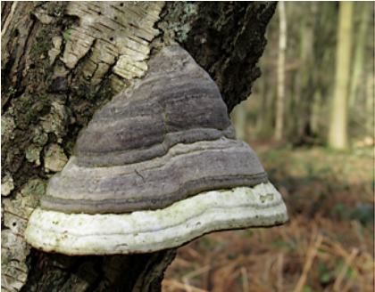
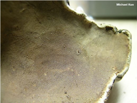
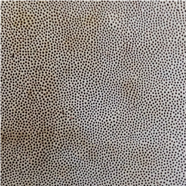
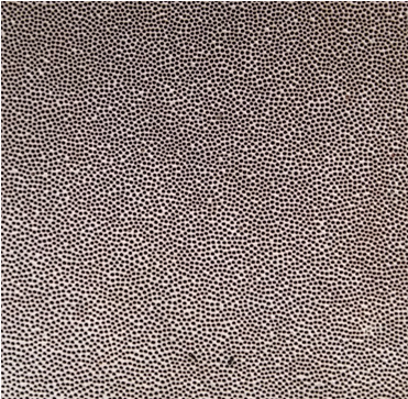
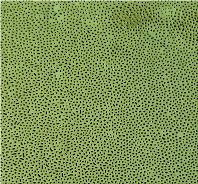
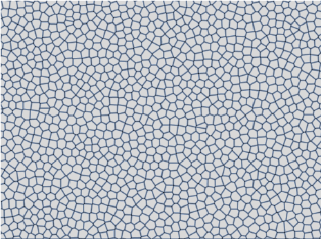
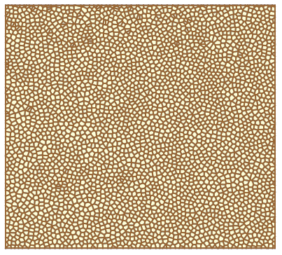
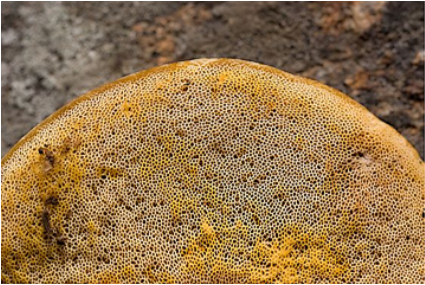
Here are well known Fomes fomentarius or "tinder polypore" mushroom, and rough image of it's bottom surface with pores (Michael Kuo photo): Here are fragments of my own photos with better resolution: and Voronoi mesh of detected pores: Obviously revealed pattern is nor grid, nor pure random, nor honeycomb-like packing.Pores are evenly distributed with roughly constant distances between neighbors.But what does it mean exactly? Is there some mathematical construct behind it?
Biological background
Biological background
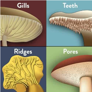
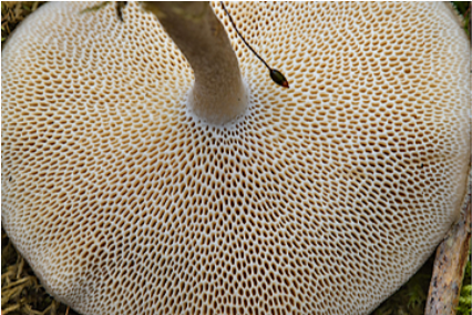
(From realmushrooms.com)Beneath the cap of many common mushrooms, you’ll find either gills (also known as lamellae), pores, ridges, or teeth: These are the parts of a mushroom’s anatomy that produce and release spores. Boletes and polypores are two common types of mushrooms that are known to have pores (Alexey Sergeev photo): On the one hand, spores should be packed as compact as possible. On the other hand, for their normal development they need enough space.So it looks like kind of blue noise structure.
Math background
Math background
It seems strange to many that neither random points nor periodic lattice are not optimally evenly equidistributed sets.
For the grid, the problem is that samples will never fall into a range smaller than grid step.
For pure white noise, sample points can clump together and leave arbitrarily large empty spaces.
There are many ways to generate evenly distributed samples, for example low discrepancy sequences, blue noise algorithms etc.
Image processing
Image processing
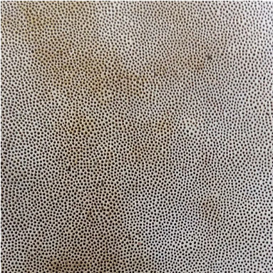
With Mathematica functions like EdgeDetect and MorphologicalComponents we can process the image and get the coordinates of the centers.
After run first code cell initializes the entire notebook, it takes 2-3 sec.
In[]:=
image=
;
In[]:=
ClearAll[poresDetect];poresDetect[img_,t1_,t2_]:=With[{newImg=Thinning@EdgeDetect[MorphologicalBinarize[img,{t1,t2}],1]},ComponentMeasurements[{newImg,MorphologicalComponents@newImg},"Centroid"]〚All,2〛];
Distributions for compare
Distributions for compare
Helper function to show samples
In[]:=
(*Переменныйразмерточек*)showPoints[arr_,size_]:=Labeled[Graphics[{LightBrown,Rectangle[],PointSize3/Length@arr,Brown,Point@arr},ImageSizesize],Length@arr];
From many evenly distributed and low-discrepancy pattern generators we choose some representative examples.
◼
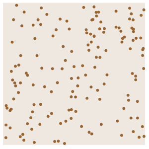
Random points
In[]:=
ClearAll[rndSamples];rndSamples[num_]:=RandomReal[{0,1},{num,2}];
In[]:=
showPoints[rndSamples[150],150]
Out[]=
150 |
In[]:=
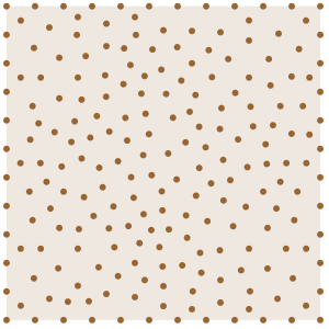
ClearAll[dsrSamples];dsrSamples[num_]:=MeshCoordinates@DiscretizeRegion[Rectangle[],MaxCellMeasure{"Area"0.8/num}];
In[]:=
showPoints[dsrSamples[200],150]
Out[]=
211 |
In[]:=
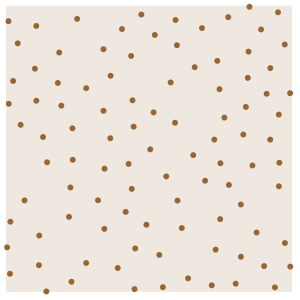
ClearAll[hppSamples];hppSamples[num_]:=RandomPointConfigurationHardcorePointProcess50num,0.8
num
,2,Rectangle[],Method->{"MCMC","LengthOfRun"5*10^4}1,1;In[]:=
showPoints[hppSamples[100],150]
Out[]=
98 |
◼
The more rate number of iterations rate, the more regular the resulting configuration.
rate = 0 returns purely random points, for rate > 20 degree of deviation from the centers less than ,
but it takes some time.
rate = 0 returns purely random points, for rate > 20 degree of deviation from the centers less than
-3
10
but it takes some time.
◼
If the parameter rnd < π is used the Fibonacci test points with randomness rnd.
If rnd > π, purely random tests are used.
If rnd > π, purely random tests are used.
Properties to compare
Properties to compare
There are a huge number of criteria and methods of examine and evaluation samples distributions.
We will consider three chosen.
We will consider three chosen.
Data
Data
Firstly we get data from images and define roughly number of samples.
Since the data is very large, this notebook will contain all the necessary functions but only with three selected data examples.
The final plots are inserted from a special notebook for calculations.
Since the data is very large, this notebook will contain all the necessary functions but only with three selected data examples.
The final plots are inserted from a special notebook for calculations.
Illustrative calculations we will conduct for fungi samples and (imho) closest candidates:
Lloyd relaxation sampling with 11 iterates and Poisson disk process with randomness 0.6
Lloyd relaxation sampling with 11 iterates and Poisson disk process with randomness 0.6
It takes 8-10 sec
Voronoi Statistics
Voronoi Statistics
Voronoi diagram is well-known method for representing and studying mathematical and natural structures.
◼
Areas of Voronoi cells
Curiously, all examples look almost identical.
But as we shall see, there are fundamental differences between them!
But as we shall see, there are fundamental differences between them!
Here are the histograms for all the examples collected on a large number of data
(~ 15 000 samples)
Next labels are used here and further:
Lloyd 2, 6, 12 — samples of Lloyd relaxation process with given number of iterations
Hardcore — Hardcore point process
Fungi — fungi pores detected coordinates
Discretize — MeshCoordinates of DiscretizeRegion built-in function
PoissonF 0.1, 0.4 — Poisson disk process with Fibonacci method test points with given randomness
PoissonR — original Poisson disk sampling
◼
Voronoi Entropy
Wolfram Community member Jessica Alfonsi suggested using Voronoi entropy of a mesh as a numerical estimate of similar configurations . Here we will calculate a few examples.
It may takes 50-60 sec!
Pair correlation function
Pair correlation function
Radial distribution (or pair correlation) fuction describes how density varies as a function of distance from a reference particle.
It is usually determined by calculating the distance between all particle pairs and binning them into a histogram. The histogram is then normalized with respect to an ideal gas, where particle histograms are completely uncorrelated.
We will need DistanceMatrix that is quickly and efficiently computed by Mathematica:
and special function
Get all possible distances between points for each example:
Select the relevant radii set:
Density variance
Density variance
To calculate this parameter, select samples that are no closer to the rMax to border.
This parameter is not relevant for too small radii.
This parameter is not relevant for too small radii.
It can be seen that (for the relevant values of radii) pore distribution of the fungus and the distribution of the Poisson disc are like a power law, but the Lloyd distribution deviates from it.
Let's try to find a simple fitting.
It is important to understand that the exponent β plays a crucial role in understanding the nature of phenomena.
Let's try to find a simple fitting.
It is important to understand that the exponent β plays a crucial role in understanding the nature of phenomena.
These are log-log plots for different distributions with more samples:
Conclusion
Conclusion
Although it’s easy to find mathematical patterns similar to the pore distribution of a tinder polypore,
(both visually and by selected numerical parameters)
it is not possible to really and fully match natural pattern.
(both visually and by selected numerical parameters)
it is not possible to really and fully match natural pattern.
Poisson Disk Sampling Minimized
Poisson Disk Sampling Minimized
CITE THIS NOTEBOOK
CITE THIS NOTEBOOK
Exploring fungi pores pattern and comparing with some known distributions
by Denis Ivanov
Wolfram Community, STAFF PICKS, June 20, 2024
https://community.wolfram.com/groups/-/m/t/3196910
by Denis Ivanov
Wolfram Community, STAFF PICKS, June 20, 2024
https://community.wolfram.com/groups/-/m/t/3196910