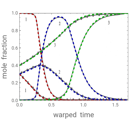
We propose to study the Batch Rectification of hexane, heptane and octane mixture at atmospheric pressure.Reflux ratio is 5 and number of theoretical stages is 7.The method of solution is based on Doherty and Malone’s textbook Conceptual Design of Distillation Systems page 395. It uses constant molar overflow assumption to get the equation of the operating line. The method also relates the composition of the still and distillate thanks to the overall and components quasi-steady-state material balances. The solution given here uses equilibrium relationships, operating lines and Dalton's law to relate the liquid-phase and vapor-phase compositions as well as the temperatures for a given initial still composition. Finally, NDSolve is used to solve the differential algebraic system of equations. We plot the still and distillate compositions versus the warped time and compare our result with Figure 9.4a given in Ref. 1.Still initial composition: %30% Hexane, 30% Heptane and 40% Octane.
Total Pressure
In[]:=
P=101.325;
Reflux ratio
In[]:=
r=5.;
Vapor Pressure of Pentane (component 1), Hexane (component 2), Heptane (component 3) and Octane (component 4).
In[]:=
PS[1,i_,t_]:=Exp[70.4265-6055.60/T[i,t]-8.37865Log[T[i,t]]+6.6166610^-6T[i,t]^2];PS[2,i_,t_]:=Exp[78.3285-6947.00/T[i,t]-9.44866Log[T[i,t]]+6.4748110^-6T[i,t]^2];PS[3,i_,t_]:=Exp[86.9970-7890.60/T[i,t]-10.6255Log[T[i,t]]+6.4744110^-6T[i,t]^2];
Normal boiling temperature (in Kelvin) of pentane, hexane, heptane and octane
In[]:=
FindRoot[PS[1,i,t]P,{T[i,t],300}]
Out[]=
{T[i,t]342.384}
In[]:=
FindRoot[PS[2,i,t]P,{T[i,t],300}]
Out[]=
{T[i,t]371.803}
In[]:=
FindRoot[PS[3,i,t]P,{T[i,t],300}]
Out[]=
{T[i,t]399.08}
Operating Line
In[]:=
Op[i_,n_,t_]:=y[i,n-1,t]r/(r+1)x[i,n,t]+1/(r+1)xD[i,t]
Raoult’s Law
In[]:=
Ra[i_,n_,t_]:=y[i,n,t]x[i,n,t]PS[i,n,t]/P
Dalton Law
In[]:=
Da[n_,t_]:=PSum[x[i,n,t]PS[i,n,t],{i,1,3}]
Forming the system of equations to be solved by FindRoot to get the initial compositions and temperature profiles in the batch rectifier
In[]:=
Sys3=Table[Op[i,n,t],{i,1,3},{n,1,7}];Sys4=Table[Ra[i,n,t],{i,1,3},{n,0,7}];Sys5=Table[Da[n,t],{n,0,7}];SystemSS=Flatten[Join[Sys3,Sys4,Sys5,Table[y[i,7,t]xD[i,t],{i,1,3}],Table[xB[i,t]x[i,0,t],{i,1,3}],{0.30xB[1,t],0.30xB[2,t],0.40xB[3,t]}]];
In[]:=
Length[SystemSS]
Out[]=
62
In[]:=
guess=Flatten[Join[Table[{{xD[i,t],0.2}},{i,1,3}],Table[{{xB[i,t],0.25}},{i,1,3}],Table[{x[i,n,t],0.2},{n,0,7},{i,1,3}],Table[{y[i,n,t],0.4},{n,0,7},{i,1,3}],Table[{{T[i,t],350}},{i,0,7}]],1]
Out[]=
{{xD[1,t],0.2},{xD[2,t],0.2},{xD[3,t],0.2},{xB[1,t],0.25},{xB[2,t],0.25},{xB[3,t],0.25},{x[1,0,t],0.2},{x[2,0,t],0.2},{x[3,0,t],0.2},{x[1,1,t],0.2},{x[2,1,t],0.2},{x[3,1,t],0.2},{x[1,2,t],0.2},{x[2,2,t],0.2},{x[3,2,t],0.2},{x[1,3,t],0.2},{x[2,3,t],0.2},{x[3,3,t],0.2},{x[1,4,t],0.2},{x[2,4,t],0.2},{x[3,4,t],0.2},{x[1,5,t],0.2},{x[2,5,t],0.2},{x[3,5,t],0.2},{x[1,6,t],0.2},{x[2,6,t],0.2},{x[3,6,t],0.2},{x[1,7,t],0.2},{x[2,7,t],0.2},{x[3,7,t],0.2},{y[1,0,t],0.4},{y[2,0,t],0.4},{y[3,0,t],0.4},{y[1,1,t],0.4},{y[2,1,t],0.4},{y[3,1,t],0.4},{y[1,2,t],0.4},{y[2,2,t],0.4},{y[3,2,t],0.4},{y[1,3,t],0.4},{y[2,3,t],0.4},{y[3,3,t],0.4},{y[1,4,t],0.4},{y[2,4,t],0.4},{y[3,4,t],0.4},{y[1,5,t],0.4},{y[2,5,t],0.4},{y[3,5,t],0.4},{y[1,6,t],0.4},{y[2,6,t],0.4},{y[3,6,t],0.4},{y[1,7,t],0.4},{y[2,7,t],0.4},{y[3,7,t],0.4},{T[0,t],350},{T[1,t],350},{T[2,t],350},{T[3,t],350},{T[4,t],350},{T[5,t],350},{T[6,t],350},{T[7,t],350}}
In[]:=
Length[guess]
Out[]=
62
In[]:=
FindRoot[SystemSS,guess]
Out[]=
{xD[1,t]0.997806,xD[2,t]0.00219253,xD[3,t]1.90499×,xB[1,t]0.3,xB[2,t]0.3,xB[3,t]0.4,x[1,0,t]0.3,x[2,0,t]0.3,x[3,0,t]0.4,x[1,1,t]0.524227,x[2,1,t]0.303497,x[3,1,t]0.172276,x[1,2,t]0.732664,x[2,2,t]0.217074,x[3,2,t]0.0502619,x[1,3,t]0.865397,x[2,3,t]0.123275,x[3,3,t]0.0113276,x[1,4,t]0.935681,x[2,4,t]0.0620808,x[3,4,t]0.002238,x[1,5,t]0.970216,x[2,5,t]0.0293684,x[3,5,t]0.000415383,x[1,6,t]0.986617,x[2,6,t]0.0133085,x[3,6,t]0.0000746078,x[1,7,t]0.994269,x[2,7,t]0.00571824,x[3,7,t]0.0000129105,y[1,0,t]0.603157,y[2,0,t]0.253279,y[3,0,t]0.143564,y[1,1,t]0.776854,y[2,1,t]0.18126,y[3,1,t]0.0418852,y[1,2,t]0.887465,y[2,2,t]0.103095,y[3,2,t]0.00943997,y[1,3,t]0.946035,y[2,3,t]0.0520994,y[3,3,t]0.00186532,y[1,4,t]0.974814,y[2,4,t]0.0248391,y[3,4,t]0.00034647,y[1,5,t]0.988482,y[2,5,t]0.0114559,y[3,5,t]0.0000624907,y[1,6,t]0.994858,y[2,6,t]0.00513063,y[3,6,t]0.0000110762,y[1,7,t]0.997806,y[2,7,t]0.00219253,y[3,7,t]1.90499×,T[0,t]366.197,T[1,t]355.335,T[2,t]348.555,T[3,t]345.22,T[4,t]343.681,T[5,t]342.973,T[6,t]342.646,T[7,t]342.496}
-6
10
-6
10
Integration using NDSolve.
In[]:=
System2=Flatten[Join[Sys3,Sys4,Sys5,Table[y[i,7,t]xD[i,t],{i,1,3}],Table[xB[i,t]x[i,0,t],{i,1,3}],Table[D[xB[i,t],t]xB[i,t]-xD[i,t],{i,1,3}]]];
In[]:=
Length[System2]
Out[]=
62
In[]:=
unk=Flatten@Join[Table[xD[i,t],{i,1,3}],Table[xB[i,t],{i,1,3}],Table[{x[i,n,t]},{n,0,7},{i,1,3}],Table[{y[i,n,t]},{n,0,7},{i,1,3}],Table[{T[i,t]},{i,0,7}]]
Out[]=
{xD[1,t],xD[2,t],xD[3,t],xB[1,t],xB[2,t],xB[3,t],x[1,0,t],x[2,0,t],x[3,0,t],x[1,1,t],x[2,1,t],x[3,1,t],x[1,2,t],x[2,2,t],x[3,2,t],x[1,3,t],x[2,3,t],x[3,3,t],x[1,4,t],x[2,4,t],x[3,4,t],x[1,5,t],x[2,5,t],x[3,5,t],x[1,6,t],x[2,6,t],x[3,6,t],x[1,7,t],x[2,7,t],x[3,7,t],y[1,0,t],y[2,0,t],y[3,0,t],y[1,1,t],y[2,1,t],y[3,1,t],y[1,2,t],y[2,2,t],y[3,2,t],y[1,3,t],y[2,3,t],y[3,3,t],y[1,4,t],y[2,4,t],y[3,4,t],y[1,5,t],y[2,5,t],y[3,5,t],y[1,6,t],y[2,6,t],y[3,6,t],y[1,7,t],y[2,7,t],y[3,7,t],T[0,t],T[1,t],T[2,t],T[3,t],T[4,t],T[5,t],T[6,t],T[7,t]}
In[]:=
Length[unk]
Out[]=
62
In[]:=
init={xD[1,0]==0.997806,xD[2,0]==0.00219253,xD[3,0]==1.90499*10^-6,xB[1,0]==0.3,xB[2,0]==0.3,xB[3,0]==0.4,x[1,0,0]==0.3,x[2,0,0]==0.3,x[3,0,0]==0.4,x[1,1,0]==0.524227,x[2,1,0]==0.303497,x[3,1,0]==0.172276,x[1,2,0]==0.732664,x[2,2,0]==0.217074,x[3,2,0]==0.0502619,x[1,3,0]==0.865397,x[2,3,0]==0.123275,x[3,3,0]==0.0113276,x[1,4,0]==0.935681,x[2,4,0]==0.0620808,x[3,4,0]==0.002238,x[1,5,0]==0.970216,x[2,5,0]==0.0293684,x[3,5,0]==0.000415383,x[1,6,0]==0.986617,x[2,6,0]==0.0133085,x[3,6,0]==0.0000746078,x[1,7,0]==0.994269,x[2,7,0]==0.00571824,x[3,7,0]==0.0000129105,y[1,0,0]==0.603157,y[2,0,0]==0.253279,y[3,0,0]==0.143564,y[1,1,0]==0.776854,y[2,1,0]==0.18126,y[3,1,0]==0.0418852,y[1,2,0]==0.887465,y[2,2,0]==0.103095,y[3,2,0]==0.00943997,y[1,3,0]==0.946035,y[2,3,0]==0.0520994,y[3,3,0]==0.00186532,y[1,4,0]==0.974814,y[2,4,0]==0.0248391,y[3,4,0]==0.00034647,y[1,5,0]==0.988482,y[2,5,0]==0.0114559,y[3,5,0]==0.0000624907,y[1,6,0]==0.994858,y[2,6,0]==0.00513063,y[3,6,0]==0.0000110762,y[1,7,0]==0.997806,y[2,7,0]==0.00219253,y[3,7,0]==1.90499*10^-6,T[0,0]==366.197,T[1,0]==355.335,T[2,0]==348.555,T[3,0]==345.22,T[4,0]==343.681,T[5,0]==342.973,T[6,0]==342.646,T[7,0]==342.496};
In[]:=
SYS=Join[System2,init];
In[]:=
Length[SYS]
Out[]=
124
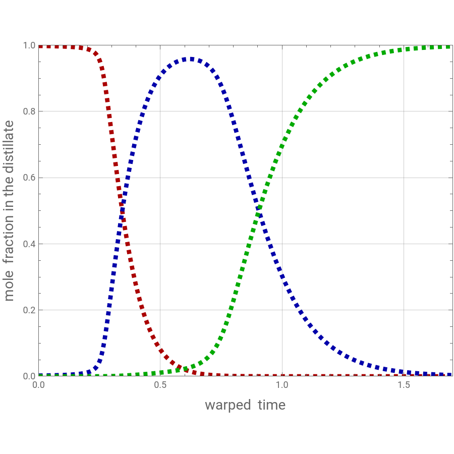
Distillate mole fraction of pentane, hexane, heptane and octane versus warped time.
Components appear in distillate in order of volatility (pentane first and octane last).
Components appear in distillate in order of volatility (pentane first and octane last).
In[]:=
sol=Quiet@NDSolve[SYS,unk,{t,0,1.6},AccuracyGoal10];
Composition in the distillate versus warped time.
Hexane = component 1 (Red Curve)
Heptane = component 2 (Blue Curve)
Octane = component 2 (Green Curve)
Hexane = component 1 (Red Curve)
Heptane = component 2 (Blue Curve)
Octane = component 2 (Green Curve)
In[]:=
p1=Plot[{xD[1,t]/.sol,xD[2,t]/.sol,xD[3,t]/.sol},{t,0,1.7},PlotRange{{0,1.7},{0,1}},FrameTrue,GridLinesAutomatic,ImageSize450{1,1},AspectRatio0.8,PlotStyle{{Thickness[0.0105],Dashed,Darker@Red},{Thickness[0.0105],Dashed,Darker@Blue},{Thickness[0.0105],Dashed,Darker@Green}},FrameLabel{Style["warped time",14],Style["mole fraction in the distillate",14]}]
Out[]=
Composition in the still versus warped time.
Hexane = component 1 (Red Curve)
Heptane = component 2 (Blue Curve)
Octane = component 2 (Green Curve)
Hexane = component 1 (Red Curve)
Heptane = component 2 (Blue Curve)
Octane = component 2 (Green Curve)
Temperature (in °C) of the distillate (blue curve) and the still (red curved).
Notice the three plateaux in the distillate temperature curve, which correspond to purified component exiting the rectifier.
Notice the three plateaux in the distillate temperature curve, which correspond to purified component exiting the rectifier.
Here, we benchmark our results against Figure 9.4a of Ref. 1.
Clearly, the agreement is satisfactory.
Hexane = component 1 (Red Curve)
Heptane = component 2 (Blue Curve)
Octane = component 2 (Green Curve)
Clearly, the agreement is satisfactory.
Hexane = component 1 (Red Curve)
Heptane = component 2 (Blue Curve)
Octane = component 2 (Green Curve)
Reference
Reference
◼
[1] Doherty and Malone, Conceptual Design of Distillation Systems, McGraw-Hill, 2001
CITE THIS NOTEBOOK
CITE THIS NOTEBOOK
Batch Rectification of a Ternary Mixture using NDSolve
by Housam Binous and Ahmed Bellagi
Wolfram Community, STAFF PICKS, January 29, 2024
https://community.wolfram.com/groups/-/m/t/3111537
by Housam Binous and Ahmed Bellagi
Wolfram Community, STAFF PICKS, January 29, 2024
https://community.wolfram.com/groups/-/m/t/3111537