Particle Swarm Optimization Applied to the van de Vusse Mechanism
Housam Binous
Particle Swarm Optimization Applied to the van de Vusse Mechanism
Housam Binous
Housam Binous
This notebook demonstrates a two-stage parameter estimation workflow applied to the van de Vusse reaction mechanism, a classic benchmark system in chemical reaction engineering involving four species (CA, CB, CC, CD) and three coupled nonlinear rate constants (k1, k2, k3) plus a time constant tau.
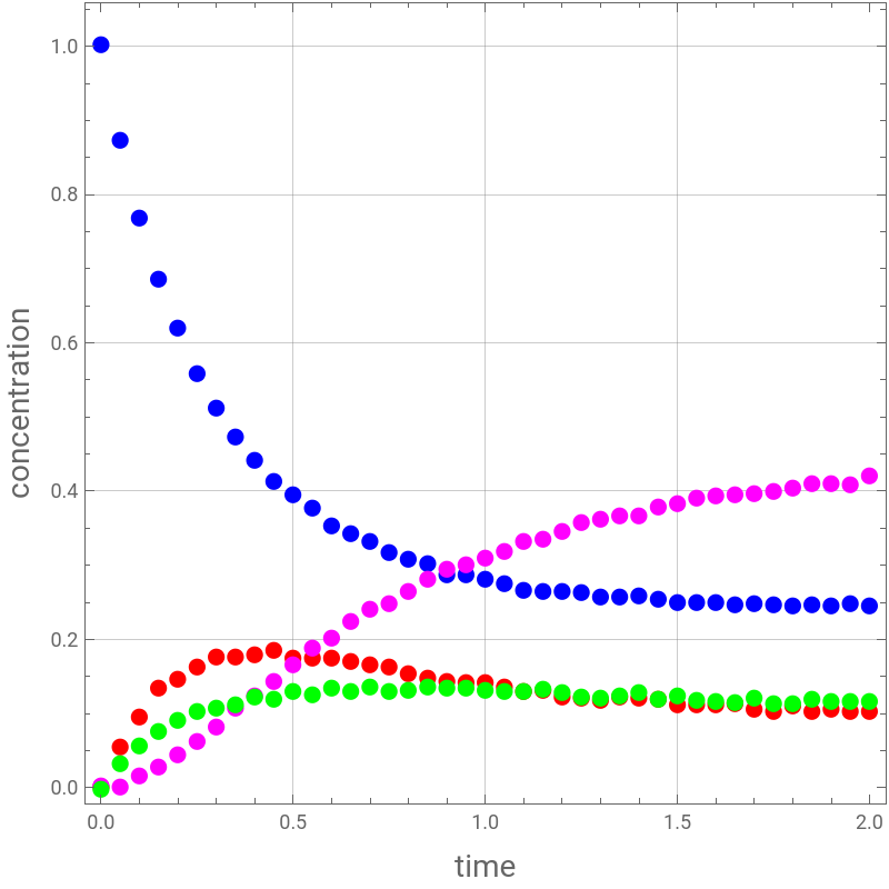
The work begins by solving the true system of ODEs using NDSolve with fixed “true” parameter values (k1E, k2E, k3E, tauE), then re-formulating the same system as a ParametricNDSolve so the model can later be evaluated at arbitrary trial parameter values. Synthetic “experimental” data is generated by sampling the true solution at discrete time points and injecting uniform random noise (controlled via a fixed seed, SeedRandom[42], for reproducibility) into all four concentration profiles, producing the noisy scatter data visible in the first plot (CA, CB, CC, CD vs. time).
The second major component defines a Fitness function that sums squared residuals between the noisy synthetic data and the parametric model’s predictions across all four species and all sample times, for any candidate parameter set {k1, k2, k3, tau}. This fitness function becomes the objective to be minimized in a custom-built Particle Swarm Optimization (PSO) routine. The PSO code includes helper functions for clipping/clamping particle positions and velocities within specified bounds, and a psoOptimize module that initializes a swarm of particles randomly within the search domain, then iteratively updates each particle’s velocity and position using the standard PSO update rule (inertia weight w, cognitive/social coefficients c1/c2, and random factors r1/r2), tracking both personal-best and global-best solutions.
The PSO is run for 300 iterations with 30 particles across a 4-dimensional search space bounded between {1,1,1,1} and {3,3,3,2}. The printed iteration log shows the loss decreasing rapidly from about 0.0036 at iteration 10 down to a plateau around 0.00131704 by iteration 100, after which it remains essentially flat through iteration 300 — indicating convergence to a global best estimate of approximately {1.34831, 2.66273, 1.54711, 1.79825} for {k1, k2, k3, tau}. This recovered parameter set is then used to re-simulate the concentration profiles and overlay them against the original noisy data, visually confirming a good fit, with the plot’s inset labels displaying the fitted k1, k2, k3, tau values alongside the achieved fitness score of 0.00132.
In the final section, the PSO result is validated by cross-checking it against Mathematica’s built-in NonlinearModelFit function. For details about this second approach see our paper (Ref. 1). The noisy data across all four species is flattened into a single long-format dataset (datanoisy), and a helper function model is defined using Through and ParametricNDSolveValue to evaluate all four concentration outputs simultaneously as a function of the parameters and time. Fitting this model to datanoisy via NonlinearModelFit yields best-fit parameters {1.35472, 2.66658, 1.5572, 1.7835}, remarkably close to the PSO solution, and the ParameterTable output provides standard errors, t-statistics, and p-values confirming the estimates are highly significant (extremely small p-values). The residual sum of squares from this fit, 0.0132768, is reported alongside a directly recomputed fitness of 0.0132768 evaluated at the NonlinearModelFit parameters — closely matching the PSO’s global best score of 0.00131704 — thereby validating that the custom PSO implementation successfully converges to essentially the same optimum as Mathematica’s professional nonlinear regression tool.
Reference:
[1] Mejri, S, Binous, H, Mahgoub, K, Bellagi, A. A model parameter estimation method using Mathematica© applied to transient chemical engineering processes.
Comput Appl Eng Educ. 2018; 26 : 1405– 1421. https://onlinelibrary.wiley.com/doi/abs/10.1002/cae.21937?msockid=17c99bec53ce6d6330e38dbb52a36ce6
In[]:=
CAi=1;tauE=1.8;k1E=1.35;k2E=2.65;k3E=1.55;sol=NDSolve[{CA'[t]1/tauE(CAi-CA[t])-k1ECA[t]-k3ECA[t]^2,CA[0]1,CB'[t]-1/tauECB[t]+k1ECA[t]-k2ECB[t],CB[0]0,CC'[t]-1/tauECC[t]+k2ECB[t],CC[0]0,CD'[t]-1/tauECD[t]+1/2k3ECA[t]^2,CD[0]0},{CA[t],CB[t],CC[t],CD[t]},{t,0,3.0}];pfunall=ParametricNDSolve[{CA'[t]1/tau(CAi-CA[t])-k1CA[t]-k3CA[t]^2,CA[0]1,CB'[t]-1/tauCB[t]+k1CA[t]-k2CB[t],CB[0]0,CC'[t]-1/tauCC[t]+k2CB[t],CC[0]0,CD'[t]-1/tauCD[t]+1/2k3CA[t]^2,CD[0]0},{CA,CB,CC,CD},{t,0,3.0},{k1,k2,k3,tau},MaxStepsInfinity,Method"StiffnessSwitching"];pfun1=CA/.pfunall;pfun2=CB/.pfunall;pfun3=CC/.pfunall;pfun4=CD/.pfunall;
noise=0.01;SeedRandom[42];noisydata1=Table[{i,Max[0,First[noise(2Random[]-1)/2+CA[t]/.sol/.ti]]},{i,0,2,0.05}];noisydata2=Table[{i,Max[0,First[noise(2Random[]-1)/2+CB[t]/.sol/.ti]]},{i,0,2,0.05}];noisydata3=Table[{i,Max[0,First[noise(2Random[]-1)/2+CC[t]/.sol/.ti]]},{i,0,2,0.05}];noisydata4=Table[{i,Max[0,First[noise(2Random[]-1)/2+CD[t]/.sol/.ti]]},{i,0,2,0.05}];p2=ListPlot[{noisydata1,noisydata2,noisydata3,noisydata4},JoinedFalse,FrameLabel->{Style["time",14],Style["concentration",14]},PlotMarkers{Style["●",Blue,12],Style["●",Red,12],Style["●",Magenta,12],Style["●",Green,12]},PlotRangeAll,FrameTrue,GridLinesAutomatic,ImageSize{400,400},AspectRatio1,PlotLegends->{"CA","CB","CC","CD"}]
Out[]=


In[]:=
Fitness[{k1_,k2_,k3_,tau_}]:=Sum[(noisydata1[[i]][[2]]-Evaluate[pfun1[k1,k2,k3,tau][t]]/.t((i-1)0.05))^2,{i,1,Length[noisydata1]}]+Sum[(noisydata2[[i]][[2]]-Evaluate[pfun2[k1,k2,k3,tau][t]]/.t((i-1)0.05))^2,{i,1,Length[noisydata1]}]+Sum[(noisydata3[[i]][[2]]-Evaluate[pfun3[k1,k2,k3,tau][t]]/.t((i-1)0.05))^2,{i,1,Length[noisydata1]}]+Sum[(noisydata4[[i]][[2]]-Evaluate[pfun4[k1,k2,k3,tau][t]]/.t((i-1)0.05))^2,{i,1,Length[noisydata1]}];SwarmDim=4;(*4Dproblem*)(*upperandlowerboundsfothesearchdomain*)FitnessLB={1,1,1,1};FitnessUB={3,3,3,2};c1=1.42;c2=1.42;w=0.72984;(*psoparameters*)
In[]:=
Clear[k1,k2,k3,tau]
PSO code
In[]:=
(*clipeachCOLUMNofamatrixagainstitsownscalarbound*)clipMatrix[mat_,lbv_,ubv_]:=Transpose[MapThread[Clip[#1,{#2,#3}]&,{Transpose[mat],lbv,ubv}]];clampMatrix[mat_,vmaxv_]:=Transpose[MapThread[Clip[#1,{-#2,#2}]&,{Transpose[mat],vmaxv}]];
In[]:=
(*PSOOptimizer*)psoOptimize[lossFunc_,dim_,lb_,ub_,nParticles_:30,nIter_:100,wMax_:0.9,wMin_:0.4,c1_:1.42,c2_:1.42,vClampFrac_:0.2]:=Module[{particles,velocities,pbest,pbestScore,gbest,gbestScore,convergence={},r1,r2,scores,gbestIdx,vmax,wIter},vmax=vClampFrac*(ub-lb);particles=Transpose@Table[RandomReal[{lb[[i]],ub[[i]]},nParticles],{i,dim}];velocities=ConstantArray[0.,{nParticles,dim}];pbest=particles;pbestScore=lossFunc/@particles;gbestIdx=First@Ordering[pbestScore,1];gbestScore=pbestScore[[gbestIdx]];gbest=pbest[[gbestIdx]];Do[wIter=wMax-(wMax-wMin)*(j-1)/(nIter-1);r1=RandomReal[1,{nParticles,dim}];r2=RandomReal[1,{nParticles,dim}];velocities=wIter*velocities+c1*r1*(pbest-particles)+c2*r2*(ConstantArray[gbest,nParticles]-particles);velocities=clampMatrix[velocities,vmax];particles+=velocities;particles=clipMatrix[particles,lb,ub];scores=lossFunc/@particles;pbest=MapThread[If[#3<#2,#1,#4]&,{particles,pbestScore,scores,pbest}];pbestScore=MapThread[Min,{pbestScore,scores}];gbestIdx=First@Ordering[pbestScore,1];If[pbestScore[[gbestIdx]]<gbestScore,gbestScore=pbestScore[[gbestIdx]];gbest=pbest[[gbestIdx]];];AppendTo[convergence,gbestScore];If[Mod[j,10]==0,Print["PSO Iter ",j," Loss = ",gbestScore]];,{j,nIter}];{gbest,gbestScore,convergence}];
In[]:=
(*PSOrun*)result=psoOptimize[Fitness,SwarmDim,FitnessLB,FitnessUB,30,300];{gbest,gbestScore,convergence}=result;
PSO Iter 10 Loss = 0.0035708
PSO Iter 20 Loss = 0.00160228
PSO Iter 30 Loss = 0.00147561
PSO Iter 40 Loss = 0.00137497
PSO Iter 50 Loss = 0.00134376
PSO Iter 60 Loss = 0.00134376
PSO Iter 70 Loss = 0.00131931
PSO Iter 80 Loss = 0.00131718
PSO Iter 90 Loss = 0.00131713
PSO Iter 100 Loss = 0.00131705
PSO Iter 110 Loss = 0.00131705
PSO Iter 120 Loss = 0.00131705
PSO Iter 130 Loss = 0.00131704
PSO Iter 140 Loss = 0.00131704
PSO Iter 150 Loss = 0.00131704
PSO Iter 160 Loss = 0.00131704
PSO Iter 170 Loss = 0.00131704
PSO Iter 180 Loss = 0.00131704
PSO Iter 190 Loss = 0.00131704
PSO Iter 200 Loss = 0.00131704
PSO Iter 210 Loss = 0.00131704
PSO Iter 220 Loss = 0.00131704
In[]:=
(*Best position = {1.34831, 2.66273, 1.54711, 1.79825}
(*best score = 0.00131704*)