Abstract. The Strait of Hormuz is the world's most strategically loaded maritime chokepoint: roughly 17–21 million barrels per day of crude and condensate transit it in nominal years, around 30% of all seaborne crude (EIA WOTC, 2024). This notebook is fully runnable in Wolfram Language: every computational figure is produced by a one-line call into the accompanying Hormuz` package (community/Hormuz.wl). Five data sources, all public: the U.S. Energy Information Administration STEO + INTL + Brent series, the U.S. Treasury OFAC SDN list, and the live AISStream.io WebSocket feed.
What you will learn. By the end of this notebook you should be able to (1) read EIA's STEO production series and distinguish capacity, disruption, and realised production; (2) compute the maximum sustainable outflow of an oil chokepoint using FindMaximumFlow on a directed-graph capacity model; (3) parse and analyse a real AIS feed with GeoHistogram, GeoPath, FindClusters, and Manipulate; and (4) recognise the structural fingerprints of the OFAC-designated dark fleet in the SDN flag distribution. The same code, parameterised on a chokepoint identifier, applies to Bab-el-Mandeb, Suez, Panama, and the Singapore Strait.
0. Loading the toolkit
0. Loading the toolkit
The whole analysis is exposed through one Wolfram-language package, Hormuz`. Load it from the same directory as this notebook:
Needs["Hormuz`","Hormuz.wl"]
1. The Strait of Hormuz: geography and stakes
1. The Strait of Hormuz: geography and stakes
In this section. Where the strait is, who loads oil there, why the Traffic Separation Scheme exists, and which two pipelines provide the only real bypass. All figures drawn from Wolfram's own coastline / country data plus live EIA production numbers.
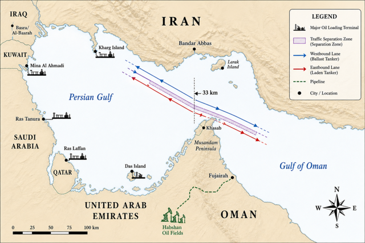
Illustration. Educational illustration (gpt-image-2). Below: the same geography rendered with Wolfram's GeoGraphics and Wolfram's own coastline data.
Roughly 30 percent of all seaborne crude oil transits the Strait of Hormuz each day in nominal years (EIA, World Oil Transit Chokepoints 2024). Eight major export terminals in the Persian Gulf load the crude, condensate, and LNG that flows out through the IMO-designated Traffic Separation Scheme (TSS) between Iran and the Musandam Peninsula of Oman – a pair of one-way lanes separated by a 2-nautical-mile buffer, originally adopted by the Inter-Governmental Maritime Consultative Organization (predecessor of IMO) in 1973 and revised in 1979, to reduce head-on collision risk in the strait's narrowest reach. Two pipelines (Saudi East-West and UAE Habshan-Fujairah) provide the only meaningful bypass capacity – their combined 6.5 mbpd is the geometric value of §3's full-closure scenario.
In WL, one call draws all of that from authoritative data:
Hormuz`HormuzGeoMap[]
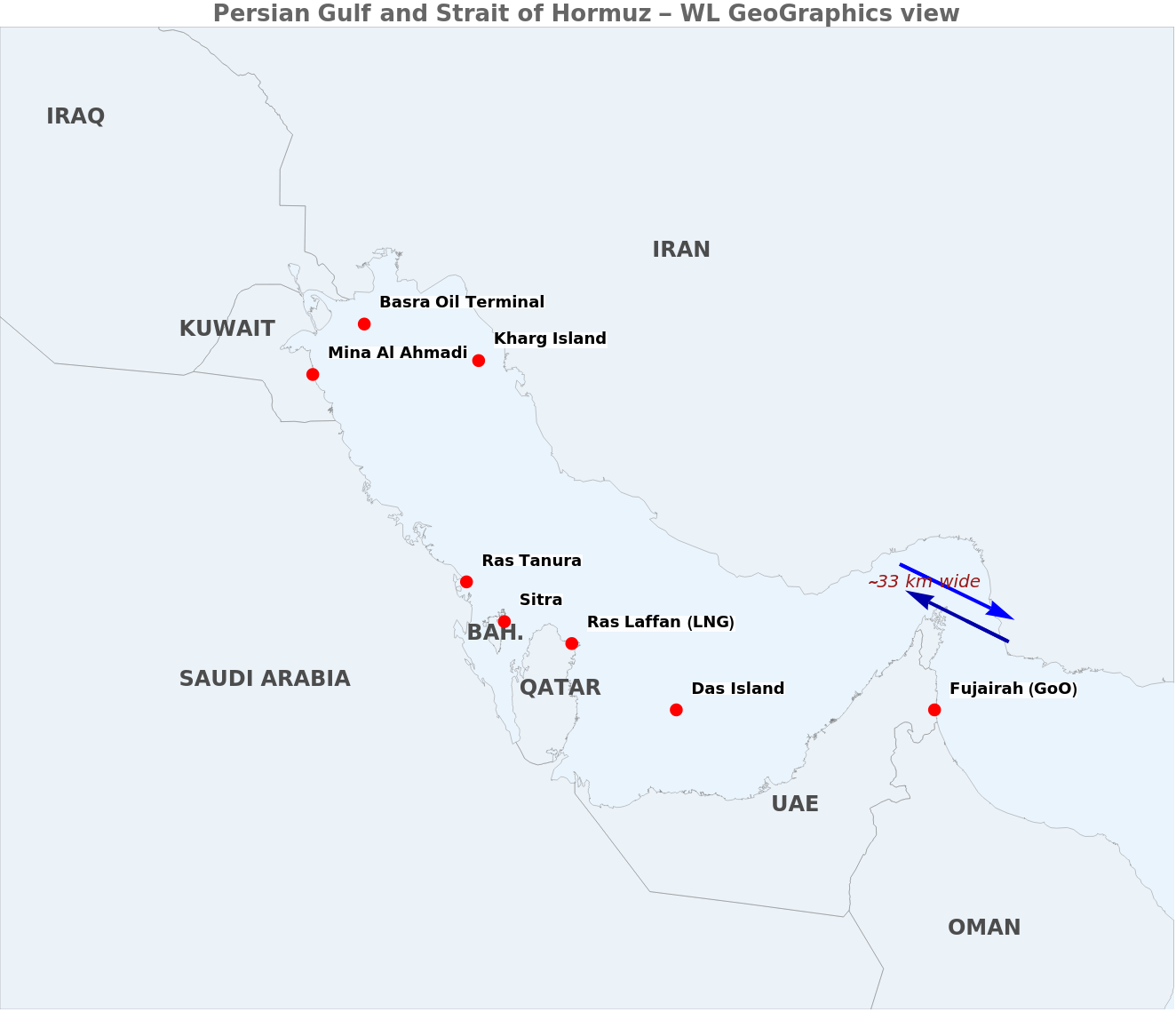
Figure. Persian Gulf and Strait of Hormuz. Country polygons from Wolfram's CountryData; eight export terminals at their published coordinates; TSS lanes drawn as GeoPath between the gate-line endpoints from chokepoints.wl. ImageSize -> Full so the figure stretches to the notebook width.
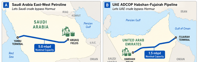
Illustration. Educational illustration (gpt-image-2). Two panels sketching the geometry of the two real Hormuz-bypass pipelines and their published nominal capacities (5.0 mbpd Saudi East-West Petroline, 1.5 mbpd UAE Habshan-Fujairah). The current per-country production numbers – including the April 2026 production drop – are in the Wolfram-computed figure immediately below.
Hormuz`OilInfrastructurePanel[]
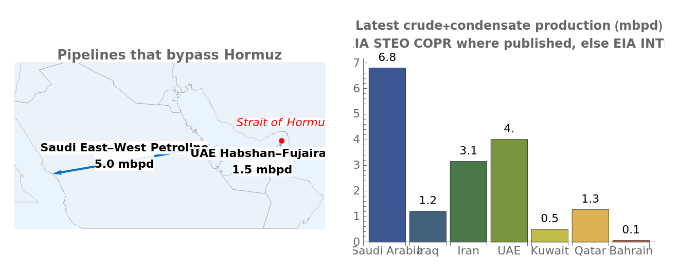
Figure. Wolfram-computed version, drawn from live EIA data. Left: GeoGraphics of the two bypass pipelines as GeoPath between published terminal coordinates. Right: actual latest per-country production – EIA STEO COPR where it is published (Iran, Iraq, Kuwait, Saudi), EIA INTL otherwise (UAE, Qatar, Bahrain). The contrast with Panel C of the illustration is the April 2026 signature: Saudi 6.8 (vs ~10 nominal), Iraq 1.2 (vs ~4.4), Kuwait 0.5 (vs ~2.75). EIA's May 2026 STEO release attributes ~10.5 mbpd of crude shut-in across these producers in April.
Takeaway. Hormuz concentrates four facts in one geographic place: ~30% of seaborne crude, a regulated IMO traffic separation scheme between Iran and Oman, and just two pipeline alternatives totalling 6.5 mbpd. Everything else in this notebook – the production data, the max-flow network, the AIS analytics, the OFAC dark-fleet structure – is downstream of these geographic and capacity facts.
2. Persian Gulf production: live data from EIA
2. Persian Gulf production: live data from EIA
In this section. How EIA's STEO series are constructed (COPC / PADI / COPR), how the April 2026 production shut-in reads off them, and how the implied outflow tracks the Brent spot price over 53 years.
All petroleum data is pulled from the U.S. Energy Information Administration. The package's loaders return Wolfram Dataset / TimeSeries objects.
EIA STEO series semantics. STEO publishes three production-related series per producer. COPC is the maximum currently-achievable production capacity net of any active unplanned disruption: in a normal month it sits as a ceiling above realised production, and a disruption event lowers it by the PADI volume. PADI is the unplanned-disruption volume itself, COPR is realised production, and COPC + PADI = nominal pre-disruption capacity. The COPC – COPR gap is not the same as PADI: in normal periods (especially for Saudi Arabia), the gap is dominated by voluntary OPEC quota restraint – capacity withheld by political decision rather than knocked out by an outage. The max-flow model in section 3 uses COPC + PADI (the network's nominal capacity, independent of OPEC quota) as edge weights, whereas the outflow series in section 2.1 uses COPR (the realised post-event production).
The April 2026 chokepoint event. EIA's May 2026 STEO release describes a coordinated Persian Gulf production shut-in. Across STEO.COPR for the four countries we splice over INTL the four-country total drops from 20.85 mbpd (Feb) to 11.65 mbpd (Apr) – a 9.2 mbpd reduction in observed crude production; EIA's narrative text cites ~10.5 mbpd including UAE/Qatar/Bahrain contributions not in the spliced series. Per-country COPR trajectories: IZ: 4.4 1.55 1.20 (Feb Mar Apr), KU: 2.56 1.15 0.50, SA: 10.5 7.30 6.80, IR: 3.39 3.25 3.15. Brent priced this in: monthly-mean spot $66.6 (Jan) $70.9 (Feb) $103.1 (Mar) $117.3 (Apr) $108.5 (May, MTD); the daily peak was $138.21 on 7 April 2026; the highest EIA daily close since the eight-day cluster of 2008 demand-cycle closes in the $138–144 band.
Hormuz`BrentOutflowPlot[]
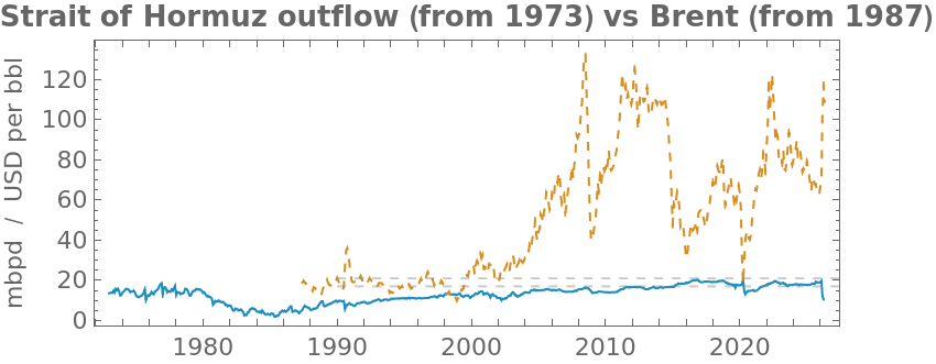


Figure. Estimated Hormuz crude+condensate outflow (derived from EIA INTL + STEO.COPR splice) and Brent monthly mean (EIA PET.RBRTE.D), 1973–present. The dashed band shows EIA's published 17–21 mbpd Hormuz-throughput range. The collapse at the right edge is the April 2026 shut-in.
Reading the 53-year figure. The outflow line traces virtually every modern oil-supply shock of consequence:
◼
1973–74. The OPEC oil embargo of October 1973 cut Persian Gulf outflow sharply, with Brent (then the marker for Arabian Gulf crudes via Suez) climbing from ~$3 to ~$12 in nominal dollars.
◼
1979–88. Iranian Revolution (1979) and the eight-year Iran-Iraq War (1980–88). Hormuz outflow drops from ~21 to ~12 mbpd; the "tanker war" phase from 1984 onward saw several hundred merchant-vessel attacks in the wider Persian Gulf, but the strait itself remained navigable and Hormuz oil never fully closed.
◼
1990–91. Iraqi invasion of Kuwait and the Gulf War. Kuwaiti production goes to zero, Iraqi production is sanctioned; Brent doubles.
◼
2003–04. Second Gulf War / U.S. invasion of Iraq. Iraqi production drops sharply but Saudi spare capacity absorbs most of the shortfall.
◼
2008. Demand-driven price spike: Chinese / Indian growth pushes Brent to its highest EIA daily close of $143.95 (3 July 2008). Hormuz outflow at the peak of the cycle, ~21 mbpd.
◼
2014–16. U.S. shale-oil output growth plus OPEC's November 2014 decision to maintain output collapses Brent from ~$100 to ~$30 over 18 months. Hormuz outflow holds, since OPEC producers are at full output.
◼
2020. COVID-19 demand collapse and the early-2020 OPEC+ pricing dispute. Brent briefly trades negative on WTI futures; Hormuz outflow drops to ~14 mbpd as OPEC+ enacts the largest coordinated production cut in the post-1973 record.
◼
April 2026. The cliff at the right edge: ~9.2 mbpd of crude production shut-in across Iran/Iraq/Kuwait/Saudi during the early-2026 Persian Gulf events and the associated Strait of Hormuz closure. Brent prints $138.21 on 7 April – within $6 of the 2008 demand-driven high, but here driven entirely by supply.
Two patterns sit on the same figure. Most supply-driven oil-price spikes in the 53-year record line up with Hormuz-outflow dips (1973–74, 1979–88, 1990–91, 2026). The 2008 peak is the exception that proves the rule: outflow was at maximum (~21 mbpd) while Brent reached $143.95, confirming the demand-driven nature of that episode. The remaining periods (2014–16 shale, 2020 demand, etc.) move on other drivers – demand, dollar, U.S. shale supply, OPEC quota – with outflow approximately steady.
Source: U.S. Energy Information Administration – STEO + INTL + Brent PET.RBRTE.D.
2.1 Daily ship traffic through the strait
2.1 Daily ship traffic through the strait
Dividing monthly outflow by typical per-transit cargo (a weighted fleet mix of VLCC 60% / Suezmax 20% / Aframax 15% / LR2 5% 1.53 mbbl per loading) yields a derived count of outbound-laden crude + condensate tanker loadings per day at Hormuz. The pre-event baseline through January and February 2026 sits at ~12.4–12.9 loadings/day; the late-February 2026 Strait of Hormuz closure shows up cleanly in the March (~7.9) and April (~6.9) data. EIA's World Oil Transit Chokepoints report cites ~14 tankers/day on the same basis with somewhat higher outflow assumptions (~21 vs. our ~19 mbpd net of pipelines).
Reconciliation to published "50–60 tanker transits/day" figures. The number above (~12 loadings/day) is a much smaller scope than the 50–60-per-day numbers commonly cited by Lloyd's List Intelligence, Reuters, and U.S. Navy 5th Fleet briefings. Building up to that number:
◼
~12 outbound-laden crude+condensate tanker loadings/day (this notebook)
◼
+12 ~25 tanker movements/day once you count the inbound ballast return that each loaded outbound implies
◼
+~15 ~40 with product + chemical tankers each way (Persian Gulf exports ~5–8 mbpd of refined products and chemicals; an LR2 carries ~0.5 mbbl)
◼
+~8–15 ~50–55 with LNG carriers (Qatar exports ~77 Mt/yr LNG → ~3–4 LNG-carrier loadings/day each way at the ~70 kt fleet-average cargo; the Q-Max class itself carries ~120 kt and so contributes ~1.8 outbound loadings/day) and LPG carriers (Saudi/Kuwait/UAE)
◼
+~5–10 ~55–65 all-tanker movements/day, matching the published 50–60-per-day figures
In short: the 12.4 number in this notebook is intentionally narrow and apples-to-apples with EIA's WOTC methodology. The published vessel-transit numbers count all tanker movements in both directions across all cargo types; multiplying our ~12 by ~4-5 reproduces that scope.
Data-completeness note. EIA STEO publishes monthly current-production COPR for Iran, Iraq, Kuwait, and Saudi Arabia only. UAE / Qatar / Bahrain production is available only via EIA INTL, which lags by ~3 months and stops at January 2026. Our estimator forward-fills the last INTL value for those three producers through the COPR window, so their contribution to the Feb-Apr 2026 figures is held at the Jan 2026 level. That is why February reads ~normal in our series even though the disruption began at month-end: it hit the Big-Four producers in the last days of February (a small fraction of the monthly aggregate) and only materialises in the March monthly figure.
Figure. Strait of Hormuz – derived daily tanker traffic, last 5 years. The Jan-Feb 2026 plateau at ~12-13 tankers/day is the pre-event baseline; the late-February 2026 Strait-of-Hormuz closure drops the implied traffic to ~7.9 in March and ~6.9 in April, all without any AIS data.
Takeaway. EIA's three-letter codes (COPC / PADI / COPR) carry exact semantics that matter when interpreting any oil-supply story. Capacity is not production, disruption is not the same as the capacity-production gap (OPEC quota fills that gap in normal times), and the early-2026 production collapse reads off all three series consistently. The implied tanker count in §2.1 (~12 loadings/day) is one slice of a multi-vessel, multi-cargo picture that reconciles to ~55–65 movements/day in published shipping-industry counts.
3. The capacity model – max-flow on the chokepoint graph
3. The capacity model – max-flow on the chokepoint graph
Illustration. Educational illustration (gpt-image-2). Below: the same network as a Wolfram Graph.
In this section. We translate the geography of section 1 into a directed-graph capacity network and use Wolfram's FindMaximumFlow to compute the maximum sustainable outflow under baseline and four disruption scenarios. The graph is the chokepoint reduced to its minimum sufficient topology; the max-flow value is the theoretical ceiling on what the strait could carry in each scenario.
Node legend (read before the figure). The graph has five classes of node. SOURCE is a synthetic supersource feeding every producer at unlimited capacity; SINK absorbs everything that leaves the Gulf of Oman. prod_<X> is the nominal capacity of producer X (live COPC + PADI from STEO for IR/IQ/KU/SA; fixed nominal values of 4.0 / 1.4 / 0.2 mbpd for UAE / Qatar / Bahrain, matching the EIA INTL crude+condensate series in recent years). term_<X> is the loading-terminal node – in this simplified model each producer routes to a single composite terminal. PG_marshal is the Persian Gulf marshalling area where outbound traffic queues before entering the TSS. TSS_west / TSS_sep / TSS_east split the Strait of Hormuz traffic separation scheme into three serial nodes; the split lets us scale westbound/separator/eastbound capacities independently to represent localised mine threat or vessel-incident closures. GoO is the Gulf of Oman side of the strait.
Edge capacities come from three sources. Producer edges (SOURCE prod term PG_marshal) use live EIA STEO COPC + PADI (nominal pre-disruption capacity) for IR/IQ/KU/SA, and fixed nominal values of 4.0 / 1.4 / 0.2 mbpd for UAE / Qatar / Bahrain (chosen to match EIA INTL crude+condensate production in recent years). Pipeline bypass edges (prod_SA SINK at 5.0 mbpd for Saudi East-West Petroline; prod_AE SINK at 1.5 mbpd for UAE Habshan-Fujairah) come directly from EIA's World Oil Transit Chokepoints 2024 publication. TSS lane capacities (12 mbpd per direction) are a modelling parameter calibrated so the baseline max-flow lands inside EIA's published 17–21 mbpd Hormuz throughput band; they are not an EIA primary series.
Figure. Hormuz capacity network. Producer + terminal + PG_marshal + TSS (west/sep/east) + GoO + sink nodes; edges carry nominal capacity (mbpd) from EIA STEO COPC + PADI plus the two EIA-published pipeline capacities.
Baseline vs current throughput. The 18.5 mbpd baseline max-flow below is the network's nominal capacity – what the chokepoint could carry if every producer ran at full COPC + PADI. The actual flow in April 2026 (section 2.1) is around 10.5 mbpd, which is much smaller – not because the network capacity shrank, but because the upstream producers shut in. Capacity is the ceiling; throughput is what is currently moving.
Wolfram's FindMaximumFlow computes the max sustainable outflow under each disruption scenario:
Figure. Max-flow values per scenario (mbpd). Baseline = full COPC+PADI through all edges, lands inside the EIA-published 17–21 mbpd Hormuz band by construction. Full TSS closure leaves 6.5 mbpd via the two pipeline bypasses, matching EIA's published bypass capacity sum.
Figure. Disruption scenarios visualised. Baseline 18.5; 30% mine threat 14.9; 50% casualty 12.5; full TSS closure 6.5 (pipelines only). The cliff between the 50%-casualty and full-closure scenarios is the geometric value of the pipeline bypass: it accounts for ~35% of nominal capacity, which is exactly the engineering rationale for building the bypass pipelines.
Takeaway. Even with the TSS at zero, the network sustains 6.5 mbpd through the two pipelines – roughly Singapore's daily fuel import. The implication is not that a Hormuz closure would be inconsequential (it would still remove ~12 mbpd from the global market and price Brent in the $150+ range as the right-edge of section 2 shows), but that the world's largest oil-supply chokepoint has a ~35% engineered fallback that quietly underwrites global energy security.
Source: U.S. Energy Information Administration STEO + 'World Oil Transit Chokepoints' report.
4. The dark fleet – OFAC SDN structural analysis
4. The dark fleet – OFAC SDN structural analysis
In this section. We load today's OFAC SDN snapshot, filter to tanker vessels under Iran/Russia/Venezuela/DPRK sanctions programs, and extract the structural fingerprint of the OFAC-designated dark fleet from the flag-of-registry distribution. The dynamic AIS-based signatures (spoofing, gaps, trajectory jumps) belong to §5.
Illustration. Educational illustration (gpt-image-2) showing the four operational signatures the OFAC 2020 Maritime Sanctions Advisory associates with sanctions evasion.
The U.S. Treasury OFAC SDN list (public, updated daily) is the authoritative registry of vessels under U.S. sanctions. Today's snapshot contains 643 tanker vessels under Iran/Russia/Venezuela/DPRK sanctions programs, of which 195 currently fly the Panamanian flag – the classic flag-of-convenience reflag.
In Wolfram the SDN list is loaded as a Dataset and filtered to dark-fleet tankers via the package's LoadOFAC[] loader. The flag distribution of those tankers is the structural fingerprint of the OFAC-designated dark fleet: more than half fly Panama or Iran; the remainder are spread across a long tail of flag-of-convenience registries (Barbados, Liberia, Palau, Gabon, Cook Islands, Comoros, Cameroon) which expand and contract as IMO and OFAC publish new SDN designations and registries respond by deregistering designated vessels.
Figure. Top flags of the OFAC-listed dark-fleet tankers in today's SDN snapshot (Iran, Russia, Venezuela, DPRK sanctions programs). Panama dominates; Iran and Barbados follow. The long tail of small registries is the reflagging-of-convenience network in numbers. WL primitives: GroupBy + Counts + ReverseSort, then BarChart.
Why Panama dominates the chart. Three structural reasons. (1) Cost and speed of entry: the Panama Maritime Authority registers a ship in days for a fee on the order of low-thousands of dollars, with no in-person inspection and no requirement that the beneficial owner be Panamanian or even disclosed to the registry. (2) Limited information-sharing: Panama participates in IMO conventions but its registry data is selectively exposed; tracing beneficial ownership through the registry alone is intentionally hard. (3) Scale: Panama is the world's largest flag-of-convenience registry by deadweight tonnage, which gives a sanctioned operator camouflage – a Panama-flagged tanker is statistically unremarkable. Iran appears directly on the chart because OFAC designates Iran-flagged vessels under the IFSR (Iranian Financial Sanctions Regulations) program; those tankers never reflagged.
The long-tail dynamic. Barbados, Liberia, Palau, Gabon, Cook Islands, Comoros, Cameroon and their peers reflect a sequential-deregistration pattern. When OFAC adds a large batch of vessels under one flag, that flag's registry comes under reputational, banking, and IMO pressure to deregister them. Operators move to the next available registry; the chart's small bars are snapshots of that migration between successive OFAC actions. Over a two-year window the rank ordering of the long tail rotates noticeably while Panama's lead stays stable.
A note on reflagging detection. The four operational signatures named in the OFAC 2020 Maritime Sanctions Advisory are: AIS spoofing, AIS gaps, trajectory jumps, and flag-of-convenience reflagging. The first three are dynamic and we detect them from AIS in §5. Reflagging is structural and lives between snapshots: the same IMO number appearing under different flags across successive SDN releases. Hormuz`DarkFleetReflagged[] runs the within-snapshot test (same IMO, different flags in one file) and returns 0 hits – zero, because OFAC publishes one canonical flag per vessel per snapshot. True reflagging detection requires the historical SDN-delta series, which the package does not currently archive.
Takeaway. The OFAC SDN list, treated as a Wolfram Dataset, reveals the sanctioned-tanker fleet's structural fingerprint in one bar chart. Detecting individual vessels' operational sanctions evasion (the AIS-signature side of the story) requires AIS data, which is what §5 demonstrates.
Source: U.S. Treasury Office of Foreign Assets Control – SDN list (sdn.xml).
5. AIS demonstration: Singapore Strait
5. AIS demonstration: Singapore Strait
In this section. We work with a live multi-day capture of vessel AIS broadcasts and use it to produce eight different WL-native visualisations of real maritime traffic: a density heatmap, vessel-class breakdown, speed/course distributions, hour-of-day pattern, individual trajectories, anchorage clusters discovered by FindClusters, a live snapshot of every vessel's latest position, and an animated Manipulate scrubbing through the most recent 12 hours.
Automatic Identification System (AIS) is the mandatory maritime transponder broadcast that every vessel over 300 GT (gross tonnage, a volumetric measure of a ship's enclosed spaces) carries. Each ship transmits a 9-digit Maritime Mobile Service Identity (MMSI, assigned by the flag state's communications regulator) along with its position, course, and speed every 2–10 seconds (more often when moving), plus its name, IMO number, and ship type every six minutes. Coastal receivers and satellites pick up the broadcasts. AISStream.io is a public WebSocket service that aggregates from volunteer terrestrial receivers – dense in Europe and South-east Asia, sparse-to-nothing in the Persian Gulf, the Red Sea, and most of the Caribbean / Pacific. So the live-AIS demonstration in this notebook necessarily runs against the Singapore Strait.
That is not a tangent: Singapore is the world's busiest chokepoint (~80,000 transits / year) and the route every Hormuz-loaded tanker bound for Asian buyers takes. The OFAC dark-fleet tankers that ship-to-ship-transfer Iranian crude in the Persian Gulf show up days later in the Singapore Strait – which is where we can actually see them.
All eight figures below are computed from the same AIS capture, collected by a daemon running on a Mac mini and streamed live from the AISStream.io WebSocket service: 319,439 parsed messages spanning 46.8 hours (2026-05-17 22:21 UTC – 2026-05-19 21:10 UTC). The figures expose eight different Wolfram-language idioms for spatial / temporal / statistical / interactive analysis.
5.1 Density heatmap (GeoHistogram)
5.1 Density heatmap (GeoHistogram)
The simplest summary is where are the ships? For each 2 km × 2 km geographic cell, count the PositionReports that fell in it. Wolfram's GeoHistogram does the spatial binning natively: pass it a list of GeoPosition objects and a bin width with a unit attached, and it returns a GeoGraphics coloured by count.
What to look for: the hottest cells are the Western Petroleum and Pulau Bukom anchorages, where dozens of tankers wait their loading slot. The thin warm strip running E–W through the middle of the strait is the deep-water fairway proper – the 200-m-deep Singapore Strait Traffic Separation Scheme through which every transit must pass.
Figure. AIS PositionReport density over the Singapore Strait, 2 km cells, TemperatureMap colour function. The bright spots are anchorages; the linear warm band is the deep-water fairway. WL primitives: GeoHistogram with a Quantity-typed bin width.
5.2 Vessel-class breakdown (ShipStaticData)
5.2 Vessel-class breakdown (ShipStaticData)
AIS messages come in two main flavours: PositionReport (the fast-cadence position+heading broadcast) and ShipStaticData (slower, every 6 minutes, carries vessel name, IMO number, ship type, dimensions, destination). The ship-type field is a 100-value numeric code bucketed by IMO into broad categories: 70–79 cargo, 80–89 tanker, 60–69 passenger, etc.
Aggregating 36 hours of static-data messages tells us what kind of ships are in the strait. The classification is dominated by tankers (more than half of all classified vessels in our window) – this is the maritime-trade signature of a strait that carries one-third of seaborne crude eastward.
Figure. Vessel-class counts from ShipStaticData over the capture window. The tanker dominance reflects Singapore's twin roles as the world's largest bunkering port and the throat through which Persian Gulf crude reaches Asia. WL primitives: GroupBy + Counts on the parsed AIS Type field.
5.3 Speed and course distributions
5.3 Speed and course distributions
Two orthogonal cuts on the same PositionReport dataset – speed over ground (SOG) and course over ground (COG):
◼
SOG histogram. AIS reports speed in tenths of a knot. The histogram has two clear features: a sharp spike at 0 kn (vessels at anchor – tens of thousands of slow pings in the capture, of which we will randomly sample 3,000 for the FindClusters demonstration in §5.6 to keep the clustering tractable) and a Gaussian-ish bump centred around 6–9 knots, which is the typical Singapore-Strait fairway transit speed under pilotage.
◼
COG rose. The course rose is a polar histogram in 20° sectors, where sector length is the count of pings with that heading. The dominant arms should run roughly E (90°) and W (270°) reflecting the bi-directional fairway. Anchored vessels still broadcast their compass heading and so contribute a spread of headings – generally aligned with the dominant ENE–WSW Singapore Strait tidal axis – which forms the rose's background plateau (not a uniform disk; tidal currents weather-vane the swinging vessel into the flow).
Figure. Left: SOG histogram. The 0-kn spike is anchored vessels; the 6–9 kn lobe is the fairway. Right: COG rose plot in 20° sectors. WL primitives: Histogram, Disk-sector polar diagram with explicit colour-coded sectors.
5.4 Hourly traffic pattern
5.4 Hourly traffic pattern
Hour-of-day shows the operational rhythm of the strait. Singapore's port is busiest in the early UTC hours (which is local mid-morning to afternoon, given UTC+8 Singapore Standard Time) when daylight pilotage windows are open and container terminals run their busiest cycle. Our 46.8-hour window spans roughly 2. diurnal cycles, so the absolute counts in each hour bin are sums across multiple days; what to read off the figure is the shape (relative height across hours), not the absolute peaks.
Figure. Ping count per UTC hour, summed across all calendar days in the capture. The lower-density hours correspond to local-Singapore overnight (UTC+8 UTC 14–22 are local 22–06). WL primitives: DateValue extracts the hour from each ping's DateObject; BarChart bins.
5.5 Trajectory case studies (GeoPath)
5.5 Trajectory case studies (GeoPath)
Aggregate statistics tell us about the population. Individual trajectories tell us about the ships. We pick the three MMSI accounts (MMSI = Maritime Mobile Service Identity, the 9-digit transponder ID that ITU assigns per vessel) with the widest geographic span in the capture window and plot their tracks as GeoPath on a Singapore-Strait base. The results below are real container and car-carrier transits through the strait – you can identify the ship by its broadcast name and look up its operator on shipping-tracker sites.
The package also cross-references each MMSI against the OFAC SDN tanker IMO list via the ShipStaticData IMO field. None of the three longest-track vessels in our window is on the SDN list (those typically appear when they offload Iranian crude in the Singapore Strait anchorages – events that occur on a weekly rather than hourly cadence). If we caught one, its panel title would print in red.
Figure. The three vessels with the widest geographic span in the 46.8-hour capture window. Red = first sighting, green = last sighting; line is the GeoPath through all intermediate positions. WL primitives: GeoPath, GroupBy on MMSI, SortBy on geographic span, GeoGraphics composition.
5.6 Anchorage clusters (FindClusters)
5.6 Anchorage clusters (FindClusters)
This one is the cleanest demonstration of Wolfram's high-level analytics on real spatial data. The procedure: filter the AIS PositionReports to those whose speed-over-ground is below 1 knot (i.e. the vessel is at anchor), then hand the resulting 3,000 randomly-sampled lat-lon pairs to FindClusters. Wolfram picks the number of clusters by Bayesian information criterion, with no manual k-means tuning.
The clusters that emerge match the published anchorage zones of the Port of Singapore: Western Petroleum Anchorage, Pulau Bukom, the Sudong Special Purpose, and the eastern Working / Cruise anchorages. We did not pre-encode these zones – the algorithm discovers them from the data. This is the unsupervised-learning angle on AIS captures.
Figure. Singapore Strait anchorages, discovered by FindClusters on slow-moving pings. Each cluster is rendered in a distinct colour over the Singapore base map. WL primitives: FindClusters with Euclidean distance, MapIndexed for colour assignment, GeoGraphics composition.
5.7 Live vessel snapshot – every ship's latest reported position
5.7 Live vessel snapshot – every ship's latest reported position
All six figures above are aggregates. The most immediate question about a live AIS feed is the most obvious one: where is every ship right now?
For each unique MMSI in the capture, we take its most-recent PositionReport, look up its AIS class from the matching ShipStaticData broadcast, and plot the result as a coloured point on the Singapore Strait. The colour key sits below the figure. Every point carries a Tooltip with the vessel's MMSI, name, and class – hover over any of them in the interactive notebook to identify the ship. This is the WL equivalent of opening MarineTraffic at this exact moment.
What you should see: a dense cluster of red dots (tankers) in the Western Petroleum and Pulau Bukom anchorages, blue dots (cargo) queued along the eastern fairway approaches and at the container terminals, a smattering of green (fishing) and orange (high-speed craft) along the coast, and a sparse line of moving vessels along the main fairway running E–W through the middle of the strait.
Figure. Singapore Strait vessel snapshot: every MMSI in the AIS capture, plotted at its most-recently-reported position, coloured by AIS class (red = tanker, blue = cargo, purple = passenger, etc.). WL primitives: GroupBy + Last to pick the latest ping per vessel, GeoGraphics with StreetMapNoLabels backdrop, Tooltip primitives for interactive per-vessel inspection.
5.8 Traffic in motion – static panels and live Manipulate
5.8 Traffic in motion – static panels and live Manipulate
A single snapshot is one frame. To see traffic evolve we need multiple frames. Hormuz`AISTrafficFrames takes the most-recent 12 hours of the capture, sub-divides it into 30-minute bins, and renders four equally-spaced bins as a 2 × 2 GraphicsGrid for direct comparison.
Figure. Singapore Strait at four moments across the most-recent 12 hours of the capture (T+0.6 h, T+4.2 h, T+7.8 h, T+11.4 h). Each panel is one 30-minute bin; colour scheme matches the live snapshot in §5.7. Reading across panels shows the fairway-traffic pulse and the persistent anchorage clusters.
The full interactive scrub through every 30-minute bin is one Manipulate call away. The Input cell below is self-contained – it loads the AIS data internally, so a reader can press Shift-Enter on this cell alone without having evaluated any earlier cell first. In a fresh local notebook session the Manipulate may take ~30 s to render the first time as LoadAIS parses 319,439 ping records; subsequent slider moves are immediate. Wolfram Cloud sessions may hit the public-tier timeout on the initial load – running this cell in desktop Mathematica is the reliable option.
Note. Manipulate-driven animation of every PositionReport over the last 12 hours of the capture, binned in 30-minute slices. The slider exposes one bin at a time; AnimationRunning -> True starts playback automatically. WL primitives: Manipulate with a discrete-integer control, GroupBy on binned timestamps, the same per-class colour scheme as the snapshot. Press Shift-Enter on the cell above to render the live animation. Static PDF exports cannot render a Manipulate cell; the four-panel grid above is the static substitute.
Takeaway. Eight figures, all from the same multi-day AIS capture, each exercising a different WL primitive: GeoHistogram for spatial density, GroupBy + Counts for class breakdown, Histogram + custom polar plot for speed/course, BarChart of DateValue for hour-of-day, GeoPath for trajectories, FindClusters for unsupervised anchorage discovery, Tooltip-decorated GeoGraphics for the live snapshot, and Manipulate for the animation. Re-pointing the loader at a different bounding box yields the same eight figures for any AIS-covered chokepoint.
Source: AISStream.io free WebSocket feed; OFAC SDN cross-reference via IMO; Singapore anchorage labels from the Maritime and Port Authority of Singapore.
6. World chokepoints: generalisation
6. World chokepoints: generalisation
In this section. The same code, parameterised on a chokepoint identifier. Each of the four other major maritime chokepoints is registered in the same Wolfram data structure as Hormuz and could be swapped in via a one-line change to the analysis.
Hormuz is the strategic centrepiece, but the analytical apparatus in Hormuz` is parameterised on the chokepoint identifier. The four other major maritime chokepoints – each with its own geometry, traffic mix, and recent operational record – are registered in the same data structure.
◼
Hormuz (Persian Gulf Gulf of Oman) – the subject of this notebook. ~21 mbpd crude+condensate in nominal years; ~30% of seaborne crude. Two-pipeline bypass (5.0 + 1.5 mbpd) is the only meaningful redundancy.
◼
Bab-el-Mandeb (Red Sea Gulf of Aden) – the chokepoint between Suez and the Indian Ocean. ~9 mbpd petroleum and a substantial share of Asia-Europe container trade. From November 2023 onward, vessel attacks attributed to Houthi forces in Yemen caused many vessels to reroute via the Cape of Good Hope, adding ~10 days transit.
◼
Suez Canal (Mediterranean Red Sea) – the fixed canal handling ~10% of global maritime trade. Single-point-of-failure proven by the Ever Given grounding in March 2021 which closed the canal for six days. Egyptian sovereign revenue depends on its throughput.
◼
Panama Canal (Atlantic Pacific) – ~14,000 transits / year, increasingly water-level constrained: 2023 drought forced an unprecedented draft reduction and transit-slot auction. Tolls have set records since.
◼
Singapore Strait (Malacca Strait South China Sea) – the busiest of all five with ~80,000 transits / year, and the single chokepoint where free terrestrial-AIS coverage is dense enough to support live monitoring. This notebook uses it as the live-AIS demonstration.
All five sit in the registry as parameterised records: bounding boxes, transit-gate line segments, nominal daily-transit counts by vessel class, and an associated commodity-price series. The max-flow and macro-data analyses generalise immediately by swapping the chokepoint id. Live AIS only works where terrestrial receivers exist.
Illustration. Educational illustration (gpt-image-2) of the five major maritime chokepoints. Below: the same chokepoints rendered with Wolfram's GeoGraphics over country polygons drawn directly from CountryData[].
Figure. The five chokepoints plotted on a Wolfram-rendered world map. Country polygons come from CountryData[] (498 entries); Hormuz is highlighted in red. Each marker carries the chokepoint's display name from the registry in wolfram/chokepoints.wl, demonstrating how the same WL data structure drives the figure.
Switching the notebook to a different chokepoint is a one-line change – all the figure functions accept the chokepoint id via the package's geometry helpers. The macro-data + max-flow modelling applies to all five; live-AIS analytics only run where AIS coverage exists.
Takeaway. Chokepoint analysis generalises cleanly because the underlying objects (a bounding box, a gate line, a producer-to-sink capacity graph, an AIS feed) are the same five primitives in every case. The parameters change – Hormuz's 6.5 mbpd of pipeline bypass has no Bab-el-Mandeb analogue, Singapore has no oil-loading function – but the methodology, the WL primitives, and the analytical framework transfer verbatim.
7. Worked extensions of the pipeline
7. Worked extensions of the pipeline
In this section. Five short follow-on analyses. Each takes one analytical primitive from §§3–6 and exposes a different facet by changing one parameter or composing two of them.
7.1 Max-flow with COPR instead of COPC + PADI
7.1 Max-flow with COPR instead of COPC + PADI
In §3 the producer edges use nominal capacity (COPC + PADI). Substituting realised production (COPR) instead answers a different question: how much could currently flow even if the TSS were fully open?
Figure. Max-flow scenarios re-evaluated on COPR-based producer edges. The baseline COPR figure is bounded above by the COPC + PADI baseline (18.5 mbpd) and below by the realised April 2026 outflow because some edges downstream of the producer (TSS, PG_marshal) still cap the system. The full-TSS-closure value is unchanged at 6.5 mbpd because that scenario is bounded entirely by the two pipeline bypass capacities, independent of upstream COPR/COPC choice.
Reading the result. Baseline drops from 18.5 (COPC + PADI) to 17.25 mbpd (COPR). The 1.2 mbpd gap is COPC + PADI minus COPR – i.e. nominal capacity minus realised output. For the four STEO producers in this snapshot that gap is mostly OPEC voluntary curtailment on Saudi Arabia plus the realised-vs-nominal difference on Iraq/Kuwait/Iran following the April 2026 disruption. The pipeline-only floor stays at 6.5 mbpd: even under full TSS closure the network can still route 6.5 mbpd through the Saudi East-West and UAE Habshan-Fujairah pipelines.
7.2 Adding Bab-el-Mandeb as a downstream bottleneck
7.2 Adding Bab-el-Mandeb as a downstream bottleneck
The Saudi East-West Petroline exits at Yanbu on the Red Sea. Crude shipped from Yanbu to Asian buyers must then transit Bab-el-Mandeb (the strait at the southern end of the Red Sea) on its way to the Indian Ocean. MaxFlowResultsBAM[9.0] re-runs the network with an explicit BAM node in series with the Saudi pipeline, parameterised at the EIA WOTC ~9 mbpd BAM capacity.
Figure. Adding Bab-el-Mandeb as a downstream chokepoint on the Yanbu route. The baseline and full-TSS-closure max-flow values are unchanged at 18.5 and 6.5 mbpd because the BAM capacity (9.0 mbpd) exceeds the Saudi East-West pipeline capacity (5.0 mbpd) by a comfortable margin – BAM is not the binding constraint in this configuration.
Reading the result. BAM is downstream-binding only if its assumed capacity falls below 5.0 mbpd. The 9.0 mbpd EIA figure is the nominal BAM capacity; if Red Sea attacks were severe enough to reduce effective BAM throughput below 5 mbpd, the Saudi pipeline ceases to be useful as a Hormuz bypass during a coincident closure. The model is parameterised so a reader can try smaller BAM capacities (e.g. MaxFlowResultsBAM[3.0]).
7.3 K-means clustering vs the BIC-chosen default
7.3 K-means clustering vs the BIC-chosen default
§5.6 used FindClusters with default settings, letting Wolfram pick the cluster count via Bayesian information criterion. Constraining the algorithm to exactly k = 6 K-means clusters answers a different question: what does the strait look like if you impose six anchorage groups?
Figure. K-means clustering with k = 6 on the same slow-moving pings as §5.6. Compared with the BIC default (which typically settles on 3–4 clusters), the k = 6 partition over-segments the larger anchorages: the Western Petroleum Anchorage and Pulau Bukom may split, and the eastern working anchorages get a finer subdivision.
Reading the result. BIC-chosen clustering captures the natural anchorage zones; imposing k = 6 reveals sub-structure within them (different sub-anchorages, holding patterns, queueing zones). Neither answer is wrong; they answer different questions. The methodological point is that K-means with fixed k partitions space arbitrarily into k groups even when the natural geography only contains 3–4 clusters.
7.4 Brent / outflow cross-correlation
7.4 Brent / outflow cross-correlation
Both series are monthly. Computing the Pearson correlation at lags from -6 to +12 months tells us at what temporal offset the two series most strongly co-move. Negative lag = Brent leads outflow; positive lag = outflow leads Brent.
Figure. Pearson correlation between monthly Hormuz outflow and Brent monthly mean, lag -6 to +12 months. The 53-year series is dominated by a strong positive secular trend (both grew across the 1973–2010 period as global oil demand industrialised), so the peak |r| sits at lag = -3 months with r = 0.701.
Reading the result. A positive peak correlation at lag = -3 months means Brent's monthly mean and Hormuz outflow co-move with Brent shifted 3 months relative to outflow. Note: this is the levels correlation, which is dominated by the long-run secular growth of both series. The supply-shock correlation (high Brent → low outflow) is more clearly seen in first differences of the two series, which the reader can compute with Differences applied to the same monthly arrays.
7.5 AIS coverage by chokepoint
7.5 AIS coverage by chokepoint
§5 used the Singapore Strait for live AIS because the AISStream.io free service has dense receiver coverage there and essentially none in the Persian Gulf. AISCoverageByChokepoint makes this concrete by counting how many of the 319,439 parsed pings fall inside each of the five registered chokepoint bounding boxes.
Figure. Per-chokepoint AIS ping counts on a log scale. Singapore receives 266940 pings; the other four chokepoints receive zero or near-zero – AISStream's free terrestrial receivers cluster in Europe and South-east Asia, leaving the Persian Gulf, the Red Sea, and Panama uncovered for free users.
Reading the result. The Singapore bar towers over the others by orders of magnitude. This is the empirical reason §5 uses Singapore for the live-AIS demonstration rather than Hormuz: it is where the receivers are. A satellite-AIS feed (paid product) would invert this distribution; the chokepoint registry in wolfram/chokepoints.wl is geometry-only and would handle either receiver mix transparently.
Takeaway across §7. The five extensions all share a pattern: change one parameter of one Wolfram primitive (edge weight, edge topology, clustering method, lag, bounding box) and read off what the modified figure tells you. The combined toolkit composes more flexibly than any of the figures individually – which is the whole point of expressing the analysis as a Wolfram package.
8. References
8. References
8.1 Primary data sources
8.1 Primary data sources
◼
U.S. Energy Information Administration, Short-Term Energy Outlook, monthly publication. www.eia.gov/outlooks/steo. Bulk dumps at www.eia.gov/opendata/bulk/STEO.zip, INTL.zip, PET_IMPORTS.zip. Series referenced in this notebook: STEO.COPC_<c>.M (current capacity), STEO.PADI_<c>.M (unplanned disruption), STEO.COPR_<c>.M (current production), STEO.COPS_OPEC_R05.Q (OPEC Middle East spare). INTL.57-1-<ISO3>-TBPD.M (crude + condensate by country).
◼
U.S. Energy Information Administration, World Oil Transit Chokepoints, 2024 edition. www.eia.gov/international/analysis/special-topics/World_Oil_Transit_Chokepoints. The source for the 17–21 mbpd Hormuz throughput band and the pipeline-bypass capacities (Saudi East-West 5.0 mbpd, UAE Habshan-Fujairah 1.5 mbpd) used in the max-flow model.
◼
U.S. Energy Information Administration, Brent spot price (FOB), daily, series PET.RBRTE.D. API endpoint: api.eia.gov/v2/seriesid/PET.RBRTE.D. Daily observations from 1987-05-20; the snapshot shipped with this notebook covers through mid-May 2026.
◼
U.S. Department of the Treasury, Office of Foreign Assets Control, Specially Designated Nationals and Blocked Persons List. Daily XML feed: sanctionslistservice.ofac.treas.gov/api/PublicationPreview/exports/SDN.XML. Vessel records carry sdnType=Vessel plus an IMO number under idType=Vessel Registration Identification which lets us cross-reference against AIS ShipStaticData broadcasts.
◼
AISStream.io, Real-time AIS WebSocket service. wss://stream.aisstream.io/v0/stream. Aggregates from volunteer terrestrial AIS receivers; free tier; bounding-box and message-type filtering server-side. Documentation: aisstream.io/documentation.
◼
Maritime and Port Authority of Singapore, Anchorage information. www.mpa.gov.sg/port-marine-ops/marine-services/anchorages. The reference for the labels (Western Petroleum, Pulau Bukom, Sudong, Changi, etc.) that match the FindClusters output in section 5.6.
8.2 Standards and regulatory references
8.2 Standards and regulatory references
◼
International Maritime Organization, Ships' Routeing (multi-volume publication; current edition 2019 with subsequent amendments). The authoritative compilation of all IMO-adopted routeing measures, including the Strait of Hormuz two-lane traffic separation scheme. The Hormuz TSS was originally adopted by IMCO (the predecessor of IMO) in 1973 and revised in 1979; the scheme has two one-way lanes separated by a 2-nautical-mile zone running roughly NW–SE between Iran and the Musandam Peninsula.
◼
International Telecommunication Union, Radiocommunication Sector, Recommendation ITU-R M.1371-5 (February 2014), Technical characteristics for an Automatic Identification System using time division multiple access in the VHF maritime mobile frequency band. The AIS protocol specification; defines the message types (PositionReport = type 1/2/3, ShipStaticData = type 5, etc.) we parse in this notebook. M.1371-5 is the current ITU-R revision; M.1371-6 has been under study but not yet adopted.
◼
International Maritime Organization, IMO Assembly, Resolution A.1117(30) (adopted 6 December 2017), IMO ship identification number scheme. Defines the 7-digit IMO numbers that persist through reflagging – which is exactly why OFAC indexes by IMO and the dark-fleet detector cross-references on it.
◼
U.S. Department of the Treasury, Office of Foreign Assets Control, U.S. Department of State, and U.S. Coast Guard, Sanctions Advisory for the Maritime Industry, Energy and Metals Sectors, and Related Communities (14 May 2020). The document that codified the four operational signatures of sanctions evasion (AIS spoofing, AIS gaps, ship-to-ship transfers, and falsified shipping documents) referenced in section 4.
8.4 Further reading
8.4 Further reading
◼
U.S. Energy Information Administration, The Strait of Hormuz is the world's most important oil transit chokepoint (Today in Energy, 4 June 2024). The reference statement for the ~20 mbpd / ~30% of seaborne-crude figure, and the laden-tanker count of ~14 / day that section 2.1 calibrates against.
◼
U.S. Energy Information Administration, World Oil Transit Chokepoints (most-recent revision). Source for both pipeline bypass capacities (Saudi East-West Petroline 5.0 mbpd, UAE Habshan-Fujairah 1.5 mbpd) and for the global ranking of chokepoint throughputs in section 6.
◼
International Energy Agency, Oil Market Report, monthly. Complements EIA STEO with the European/OECD view of the same production-disruption events.
◼
U.S. Department of the Treasury, Office of Foreign Assets Control, Recent Actions feed (sanctions designations and delistings). ofac.treasury.gov/recent-actions. The primary record of changes to the SDN list between snapshots; the reflagging-of-convenience and sequential-deregistration dynamics described in section 4 are most cleanly observed in this delta series.
◼
Lloyd's List Intelligence, Seasearcher vessel-tracking platform. Industry-standard tool for IMO-to-flag-history research; the reflagging-of-convenience dynamic described in section 4 is most visible in Seasearcher's historical flag-of-record series.
9. Acknowledgements
9. Acknowledgements
AIS data: AISStream.io community of contributing receiver operators. Petroleum data: U.S. Energy Information Administration. Sanctions data: U.S. Department of the Treasury OFAC.
10. Reproducibility
10. Reproducibility
This notebook is fully runnable in Wolfram Language. Two files:
◼
hormuz_chokepoint.nb
◼
– this notebook.
◼
Hormuz.wl
◼
– the accompanying package (place in the same directory).
To regenerate the underlying data CSVs (Brent, EIA bulk dumps, OFAC, AIS captures), see the project repository at github.com/mthiel74/StraightofHormuz.
Generated 2026-05-21T14:45:09 UTC by community/build_notebook.wls.
CITE THIS NOTEBOOK
CITE THIS NOTEBOOK
Strait of Hormuz: live AIS, EIA petroleum data, OFAC sanctions, and a directed-graph capacity model
by Marco Thiel
Wolfram Community, STAFF PICKS, May 21, 2026
https://community.wolfram.com/groups/-/m/t/3719828
by Marco Thiel
Wolfram Community, STAFF PICKS, May 21, 2026
https://community.wolfram.com/groups/-/m/t/3719828