ORIGINAL ARTICLE: H. Binous, M. A. Al-Harthi and A. Bellagi, Experimental and Theoretical Study of Multicomponent Batch Distillation, Computer Applications in Engineering Education Journal, 23(6), pp. 813-823, 2015. DOI: 10.1002/cae.21652
Article Abstract: We present in this pedagogical paper several important aspects of multi-component batch distillation. These later include: (1) Experimental implementation and results of a simple multi-component batch distillation; (2) Theoretical prediction of temperature and composition evolution with time; and (3) Liquid-vapor equilibrium calculations of ternary mixtures, including residue curves computations. Such study material can be easily introduced in undergraduate chemical engineering laboratory including the senior-level laboratory, called CHE 409 at King Fahd University of Petroleum & Minerals (KFUPM). The selected multi-component mixture is composed of chloroform, acetone, and methanol. This mixture is particularly interesting because it has several distillation boundaries and up to four azeotropes. During the simple batch distillation experiment, temperature of the vapor phase is measured and both the initial and final compositions are determined using Nuclear Magnetic Resonance (NMR). These experimental results are then compared to the theoretical calculations based on two approaches: (i) mass and energy balance approach (i.e, MESH equations) and (ii) residue curve.
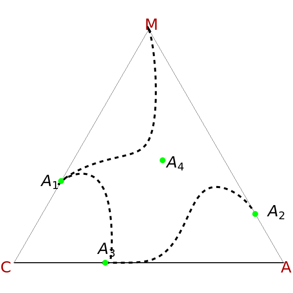
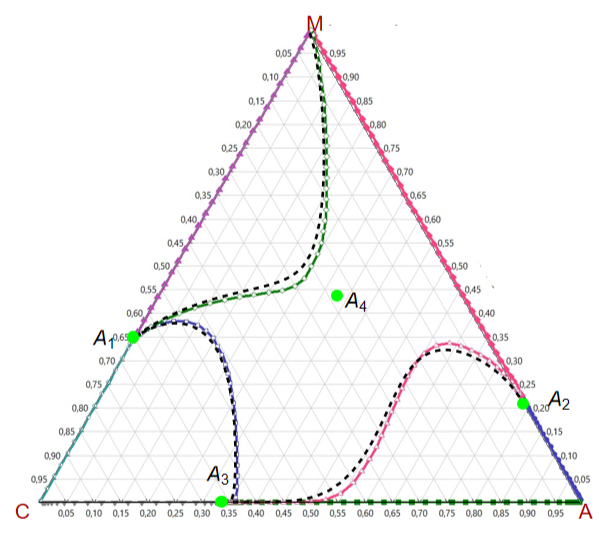
Consider a ternary mixture of chloroform, acetone, and methanol at . The vapor-liquid equilibrium (VLE) behavior is described by the modified Raoult's law with activity coefficients predicted by the Wilson model [1]. We plot three residue curves for this system on a ternary equilateral diagram. Then, we compare our data against their counterparts obtained using Aspen-Properties tools.
101.325kPa
Gas Constant (expressed in kcal/K*kmol) and Total Pressure (expressed in KPa)
In[]:=
R=1.987;P=101.325;
Vapor Pressure Using Antoine Equation : (Temperature T expressed in Kelvin)()=++T+ln(T)+ Chloroform component 1Acetone component 2Methanol component 3
ln
sat
P
i
A
i
B
i
C
i
D
i
E
i
F
i
T
In[]:=
A1=73.7058;B1=-6055.60;C1=0;D1=-8.91890;E1=7.7440710^-6;F1=2.0;A2=71.3031;B2=-5952.00;C2=0.0;D2=-8.53128;E2=7.8239310^-6;F2=2.0;A3=59.8373;B3=-6282.89;C3=0;D3=-6.37873;E3=4.6174610^-6;F3=2.0;
In[]:=
PSat1[t_]:=Exp[A1+B1/(C1+T[t])+D1Log[T[t]]+E1T[t]^F1];PSat2[t_]:=Exp[A2+B2/(C2+T[t])+D2Log[T[t]]+E2T[t]^F2];PSat3[t_]:=Exp[A3+B3/(C3+T[t])+D3Log[T[t]]+E3T[t]^F3];
Binary interaction Parameters and Activities for Wilson Model
In[]:=
l12=-506.85180;l21=116.11710;l13=-361.79440;l31=1694.02400;l23=-124.93280;l32=551.45450;
In[]:=
V1=80.7;V2=74.0;V3=40.7;(*molarvolumes*)
In[]:=
A12=V2/V1Exp[-l12/(R*(T[t]))];A13=V3/V1Exp[-l13/(R*(T[t]))];A32=V2/V3Exp[-l32/(R*(T[t]))];A21=V1/V2Exp[-l21/(R*(T[t]))];A31=V1/V3Exp[-l31/(R*(T[t]))];A23=V3/V2Exp[-l23/(R*(T[t]))];
In[]:=
GAM1[i_]:=Exp[-Log[x1[i]+x2[i]*A12+x3[i]*A13]+1-(x1[i]/(x1[i]+x2[i]*A12+x3[i]*A13)+x2[i]*A21/(x1[i]*A21+x2[i]+x3[i]*A23)+x3[i]*A31/(x1[i]*A31+x2[i]*A32+x3[i]))];GAM2[i_]:=Exp[-Log[x1[i]*A21+x2[i]+x3[i]*A23]+1-(x1[i]*A12/(x1[i]+x2[i]*A12+x3[i]*A13)+x2[i]/(x1[i]*A21+x2[i]+x3[i]*A23)+x3[i]*A32/(x1[i]*A31+x2[i]*A32+x3[i]))];GAM3[i_]:=Exp[-Log[x1[i]*A31+x2[i]*A32+x3[i]]+1-(x1[i]*A13/(x1[i]+x2[i]*A12+x3[i]*A13)+x2[i]*A23/(x1[i]*A21+x2[i]+x3[i]*A23)+x3[i]/(x1[i]*A31+x2[i]*A32+x3[i]))];
Equilibrium relations
In[]:=
y1[t_]=x1[t]PSat1[t]GAM1[t]/P;y2[t_]=x2[t]PSat2[t]GAM2[t]/P;y3[t_]=x3[t]PSat3[t]GAM3[t]/P;
Summation rule
In[]:=
x3[t_]:=1-x1[t]-x2[t];
In[]:=
sol1=Quiet@NDSolve[{D[x1[t],{t,1}]y1[t]-x1[t],D[x2[t],{t,1}]y2[t]-x2[t],(x1[t]PSat1[t]GAM1[t]+x2[t]PSat2[t]GAM2[t]+x3[t]PSat3[t]GAM3[t]-P)0,T[0]340,x1[0]0.0565,x2[0]0.1026},{x1,x2,T},{t,-80,80}];
In[]:=
sol2=Quiet@NDSolve[{D[x1[t],{t,1}]y1[t]-x1[t],D[x2[t],{t,1}]y2[t]-x2[t],(x1[t]PSat1[t]GAM1[t]+x2[t]PSat2[t]GAM2[t]+x3[t]PSat3[t]GAM3[t]-P)0,T[0]340,x1[0]0.55555,x2[0]0.277777},{x1,x2,T},{t,-80,80}];
In[]:=
sol3=Quiet@NDSolve[{D[x1[t],{t,1}]y1[t]-x1[t],D[x2[t],{t,1}]y2[t]-x2[t],(x1[t]PSat1[t]GAM1[t]+x2[t]PSat2[t]GAM2[t]+x3[t]PSat3[t]GAM3[t]-P)0,T[0]340,x1[0]0.1645,x2[0]0.545},{x1,x2,T},{t,-80,80}];
Plot of Residue Curves
Plot of Residue Curves
Azeotropes are show as green dots. This mixture presents four azeotropes, whose locations and boiling points are:
mole% | BP°C | |||
chloroform | methanol | acetone | ||
A 1 | 65.52 | 34.48 | - | 53.82 |
A 2 | - | 20.93 | 79.07 | 55.35 |
A 3 | 66.13 | - | 33.21 | 64.45 |
A 4 | 22.90 | 43.89 | 33.21 | 57.32 |
In[]:=
DATA1=Flatten[Table[{x2[t],x3[t],x1[t]}/.sol1,{t,-80,80,0.4}],1];
In[]:=
DATA2=Flatten[Table[{x2[t],x3[t],x1[t]}/.sol2,{t,-80,80,0.4}],1];
In[]:=
DATA3=Flatten[Table[{x2[t],x3[t],x1[t]}/.sol3,{t,-80,80,0.4}],1];
Loci of the Azeotropes
In[]:=
AZ1=Last@DATA1
Out[]=
{1.43882×,0.344955,0.655045}
-13
10
In[]:=
AZ2=Last@DATA3
Out[]=
{0.790708,0.209292,-2.95195×}
-13
10
In[]:=
AZ3=First@DATA2
Out[]=
{0.338703,-5.55112×,0.661297}
-17
10
In[]:=
AZ4={0.3321,0.4389,0.2290}
Out[]=
{0.3321,0.4389,0.229}
In[]:=
Pt={{2,1}/2,{0,Sqrt[3.]}/2};(*transformationfromrectangulartoequilateral*)
Our residue curves
In[]:=
p1=Show[TernaryListPlot[{DATA1,DATA2,DATA3},Joined->True,PlotStyle->{{Thick,Black,Dashed},{Thick,Black,Dashed},{Thick,Black,Dashed}},Frame->False,ImageSize->300{1,1}],Graphics[{Style[Text["",Pt.{-0.075,0.35},{-1,0}],16],Style[Text["",Pt.{0.83,0.22},{-1,0}],16],Style[Text["",Pt.{0.28,0.06},{-1,0}],16],Style[Text["",Pt.{0.35,0.43},{-1,0}],16],Green,PointSize[0.02],Point[Pt.{0.,0.35}],Point[Pt.{0.7907,0.209}],Point[Pt.{0.3387,0}],Point[Pt.{0.3321,0.4389}],Text[Style["C",16,Darker@Red],Pt.{-0.02,-0.02}],Text[Style["A",16,Darker@Red],Pt.{1.02,-0.02}],Text[Style["M",16,Darker@Red],Pt.{-0.0,1.02}]}]]
A
1
A
2
A
3
A
4
Out[]=
Mathematica versus Aspen-Properties
Mathematica versus Aspen-Properties
The same calculation using Aspen-Properties
In[]:=
IMG=
;
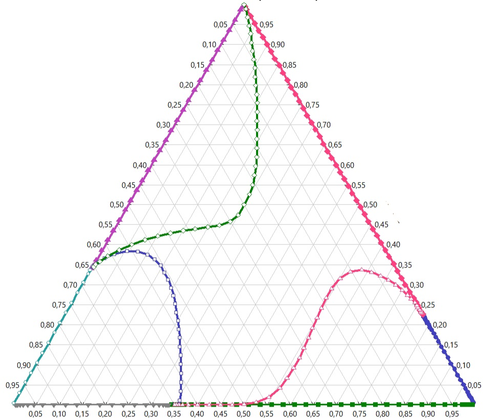
Note that the small discrepancy in the residue curves is most likely due to different sets of binary interaction parameters used for the Wilson’s model (Ref. 1)
In[]:=
Show[p1,ImageSize->450{1,1},Prolog{Raster[ImageData[IMG,DataReversedTrue],{Scaled[{-0.0225,-0.03725},{0,0}],Scaled[{1.89,1.87}/2,{0,0}]}]},ImagePadding->{{10,Automatic},{10,Automatic}}]
References
References
◼
[1] G. M. Wilson, “Vapor-Liquid Equilibrium XI: A New Expression for the Excess Free Energy of Mixing,” Journal of the American Chemical Society, 86(2), 1964 pp. 127–130.
◼
[2] H. Binous, M. A. Al-Harthi and A. Bellagi, Experimental and Theoretical Study of Multicomponent Batch Distillation, Computer Applications in Engineering Education Journal, 23(6), pp. 813-823, 2015.
CITE THIS NOTEBOOK
CITE THIS NOTEBOOK
Residue Curve Computed using Mathematica versus their Counterparts by Aspen-Properties
by Housam Binous and Ahmed Bellagi
Wolfram Community, STAFF PICKS, January 21, 2024
https://community.wolfram.com/groups/-/m/t/3107013
by Housam Binous and Ahmed Bellagi
Wolfram Community, STAFF PICKS, January 21, 2024
https://community.wolfram.com/groups/-/m/t/3107013