ABSTRACT (original article): We study four non-Newtonian fluid mechanics problems using Mathematica[R]. Constitutive equations describing the behavior of power-law, Bingham and Carreau models are recalled. The velocity profile is obtained for the horizontal flow of power-law fluids in pipes and annuli. For the vertical laminar film flow of a Bingham fluid we determine the velocity profile. Both problems involve the use of the shooting techniques because they have split boundary conditions. Since Mathematica permits symbolic computations, we determine analytical expressions of volumetric flow rates for pipe flow of the Bingham and power-law fluids. We use the built-in optimization command of Mathematica, FindMinimum, in order to find the non-Newtonian fluid model from representative data of flow rates measured under different applied pressure gradients in a horizontal pipe. These pedagogic problems are used to introduce the field of non-Newtonian fluid mechanics to students at the National Institute of Applied Sciences in Tunis. The Mathematica[R] notebooks are available from the corresponding author upon request or at Wolfram Research. (Contains 1 table and 6 figures). CITATION (original article): Binous, Housam (2007). “Introducing Non-Newtonian Fluid Mechanics Computations with Mathematica in the Undergraduate Curriculum.” Chemical Engineering Education 41(1):59–64. ISSN-0009-2479. https://www.researchgate.net/publication/237109031
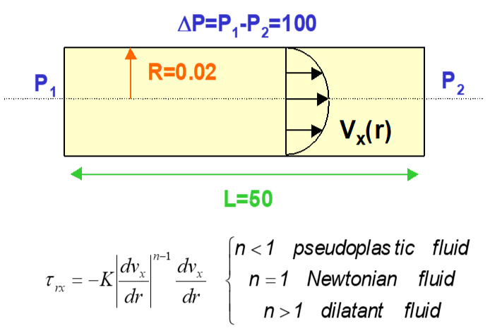
We propose to find the velocity profiles for the laminar flow of power-law fluids in a pipe (as depicted in below). Various methods are proposed: the shooting method, the orthogonal collocation technique and the analytical solution. We use the following values for the pressure difference ΔP, the exponent n, the consistency index k, the pipe length L, and radius R:
ΔP =100; L = 50; and R = 0.02
Dilatant fluid: and
Pseudo-plastic fluid: and
Dilatant fluid:
n=3.39
κ=
-6
10
Pseudo-plastic fluid:
n=0.4
κ=5×
-3
10
In[]:=
Clear[r,Ds,d,y,V,v,tau,τ,n,K]
Flow of dilatant and pseudoplastic fluids in a horizontal pipe
Flow of dilatant and pseudoplastic fluids in a horizontal pipe
Analytical Solution
v
z
n
n+1
1
n
ΔP
2KL
n+1
n
R
n+1
n
r
R
In[]:=
v
analytical
In[]:=
v
analytical
Out[]=
1+n
n
0.02
1
n
1
K
1+n
n
50.
1+n
n
r
1+n
Dilatant Fluid: solution based on the shooting technique
In[]:=
K=110^-6;n=3.39;ΔP=100;L=50;R=0.02;
In[]:=
system[Ω_]={D[r[r],{r,1}]ΔP/Lr,D[[r],{r,1}]If[[r]≥0,-([r]/K)^(1/n),(-[r]/K)^(1/n)],[10^-5]0,[10^-5]Ω};myODEsoln[Ω_]:=NDSolve[system[Ω],{,},{r,10^-5,R}]yend[Ω_?NumericQ]:=Flatten[([r]/.myODEsoln[Ω])/.rR]bc=FindRoot[yend[Ω]0,{Ω,0,0.5}][[1,2]];
τ
rx
v
x
τ
rx
τ
rx
τ
rx
τ
rx
v
x
v
x
τ
rx
v
x
In[]:=
sol1=myODEsoln[bc]
Out[]=
InterpolatingFunction,InterpolatingFunction
v
x


τ
rx

In[]:=
plt1=Plot[[r]/.sol1,{r,0.00001,R},PlotStyle{Thick,Darker@Green},Frame->True,AspectRatio->1,FrameLabel->{Style["position",14],Style["velocity",14]},GridLines->Automatic,ImageSize->350{1,1}]
v
x
Out[]=
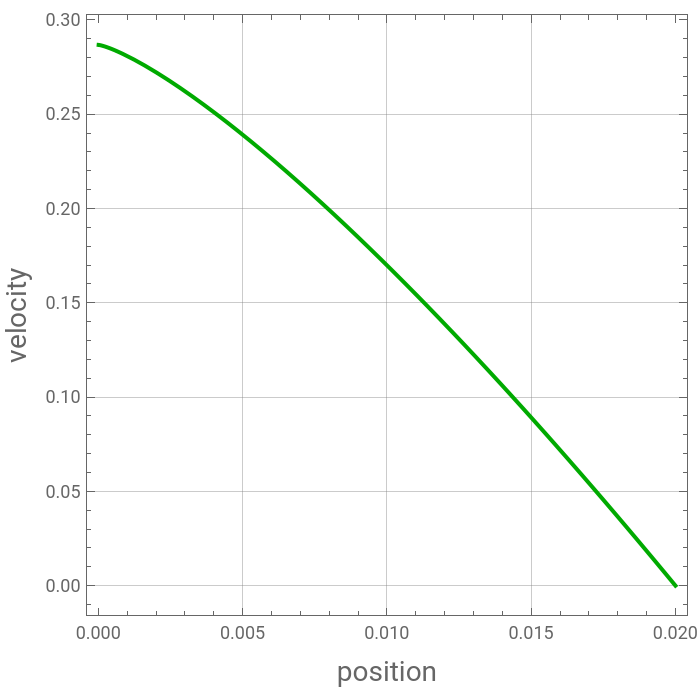
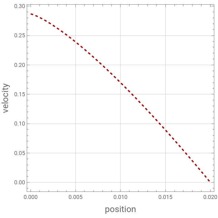
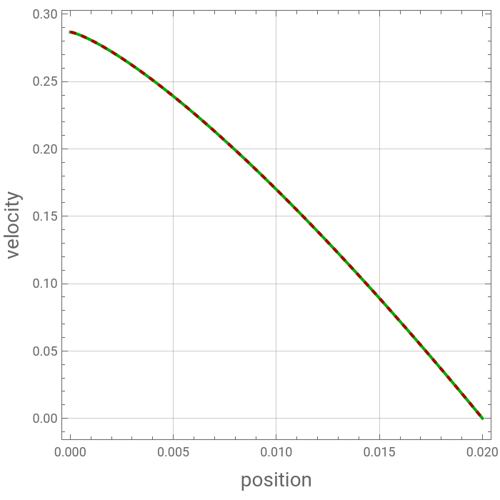
Comparing numerical result (solid line) with analytical solution (dashed curve) for dilatant fluid
In[]:=
plt2=Plot[r],{r,0.00001,R},PlotStyle{Thick,Darker@Red,Dashed},Frame->True,AspectRatio->1,FrameLabel->{Style["position",14],Style["velocity",14]},GridLines->Automatic,ImageSize->350{1,1}
v
analytical
Out[]=
In[]:=
Show[plt1,plt2]
Out[]=
Comparing analytical solution (dashed red curve) and solution (black dots) using Chebyshev Orthogonal Collocation for dilatant fluid
In[]:=
Np=40;Ds=Table[d[i,j],{i,0,Np},{j,0,Np}];d[0,0]=(2Np^2+1)/6//N;d[Np,Np]=-(2Np^2+1)/6//N;d[i_,i_]:=-y[i]/(2(1-y[i]^2));y[i_]:=Cos[iPi/Np]//N;d[j_,k_]:=If[j≠k,c[j](-1)^(j+k)/(c[k](y[j]-y[k]))];c[i_]:=If[i0||iNp,2,1];
In[]:=
V=Table[v[i],{i,1,Np+1}]//Flatten;
In[]:=
τ=Table[tau[i],{i,1,Np+1}]//Flatten;
In[]:=
r=Table[R/2(1+y[i]),{i,Np,0,-1}]
Out[]=
{0.,0.0000308267,0.000123117,0.000276301,0.000489435,0.000761205,0.00108993,0.0014736,0.00190983,0.00239594,0.00292893,0.00350552,0.00412215,0.00477501,0.0054601,0.00617317,0.00690983,0.00766555,0.00843566,0.00921541,0.01,0.0107846,0.0115643,0.0123345,0.0130902,0.0138268,0.0145399,0.015225,0.0158779,0.0164945,0.0170711,0.0176041,0.0180902,0.0185264,0.0189101,0.0192388,0.0195106,0.0197237,0.0198769,0.0199692,0.02}
In[]:=
Eq1[i_,K_,n_]:=2/R(Ds.V)[[i]]If[tau[i]≥0,-(tau[i]/K)^(1/n),(-tau[i]/K)^(1/n)];
In[]:=
Eq2[i_]:=r[[Np+2-i]]2/R(Ds.τ)[[i]]+tau[i]==r[[Np+2-i]]ΔP/L;
In[]:=
BC1=v[1]==0;BC2=tau[Np+1]==0;
In[]:=
unknowns=Flatten[Join[{Table[{V[[i]],0.5},{i,1,Np+1}],Table[{τ[[i]],0.5},{i,1,Np+1}]}],1];
In[]:=
SYS=Flatten[Join[{BC1,BC2,Table[Eq1[i,K,n],{i,2,Np+1}],Table[Eq2[i],{i,1,Np}]}],1];
In[]:=
sol=FindRoot[SYS,unknowns]
Out[]=
{v[1]-7.12878×,v[2]0.000596785,v[3]0.00228382,v[4]0.00514413,v[5]0.00905432,v[6]0.0140777,v[7]0.020072,v[8]0.0270821,v[9]0.0349486,v[10]0.0437005,v[11]0.0531635,v[12]0.0633537,v[13]0.0740852,v[14]0.0853643,v[15]0.0969974,v[16]0.108985,v[17]0.121129,v[18]0.133429,v[19]0.145687,v[20]0.157905,v[21]0.169889,v[22]0.181647,v[23]0.192995,v[24]0.203951,v[25]0.214343,v[26]0.224203,v[27]0.233374,v[28]0.241906,v[29]0.249661,v[30]0.256706,v[31]0.262924,v[32]0.268406,v[33]0.273056,v[34]0.276987,v[35]0.280127,v[36]0.282614,v[37]0.284403,v[38]0.285655,v[39]0.286359,v[40]0.286709,v[41]0.286758,tau[1]0.02,tau[2]0.0199692,tau[3]0.0198769,tau[4]0.0197237,tau[5]0.0195106,tau[6]0.0192388,tau[7]0.0189101,tau[8]0.0185264,tau[9]0.0180902,tau[10]0.0176041,tau[11]0.0170711,tau[12]0.0164945,tau[13]0.0158779,tau[14]0.015225,tau[15]0.0145399,tau[16]0.0138268,tau[17]0.0130902,tau[18]0.0123345,tau[19]0.0115643,tau[20]0.0107846,tau[21]0.01,tau[22]0.00921541,tau[23]0.00843566,tau[24]0.00766555,tau[25]0.00690983,tau[26]0.00617317,tau[27]0.0054601,tau[28]0.00477501,tau[29]0.00412215,tau[30]0.00350552,tau[31]0.00292893,tau[32]0.00239594,tau[33]0.00190983,tau[34]0.0014736,tau[35]0.00108993,tau[36]0.000761205,tau[37]0.000489435,tau[38]0.000276301,tau[39]0.000123117,tau[40]0.0000308267,tau[41]0.}
-23
10
Pseudoplastic Fluid: solution based on the shooting technique
Comparing analytical solution (dashed blue curve) and solution (black dots) using Chebyshev Orthogonal Collocation for pseudoplastic fluid
Velocity profiles for dilatant (red curve) and pseudoplastic (blue curve) fluids under equal volumetric flow assumption
Acknowledgement
Acknowledgement
Since in this laminar flow problem, we have split boundary conditions. Problem’s resolution, based on the Shooting Method, is derived based on coding developed in Mathematica by Professor Brian Higgins (University of California, Davis).
References
References
◼
J. O. Wilkes, Fluid Mechanics for Chemical Engineers, Upper Saddle River, NJ: Prentice Hall, 1999.
CITE THIS NOTEBOOK
CITE THIS NOTEBOOK
Velocity profile for laminar flow of dilatant and pseudoplastic fluids using orthogonal collocation
by André Von-Held Soares, Lizandro de Sousa Santos, Housam Binous and Ahmed Bellagi
Wolfram Community, STAFF PICKS, April 18, 2024
https://community.wolfram.com/groups/-/m/t/3160332
by André Von-Held Soares, Lizandro de Sousa Santos, Housam Binous and Ahmed Bellagi
Wolfram Community, STAFF PICKS, April 18, 2024
https://community.wolfram.com/groups/-/m/t/3160332