Introduction
Introduction
A fractal is a geometric shape containing detailed structure at arbitrarily small scales, usually having a fractal dimension strictly exceeding the topological dimension.
Problematic
Problematic
How do fractals influence the way we perceive dimensional space?
Summary
Summary
1. Menger Sponge;
2. Sierpinski triangle/pyramid;
3. Von Koch Snowflake;
4. Peano Curve.
2. Sierpinski triangle/pyramid;
3. Von Koch Snowflake;
4. Peano Curve.
Menger Sponge
Menger Sponge
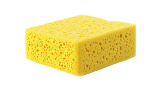
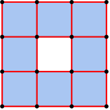
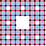
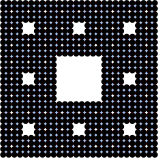
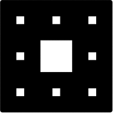
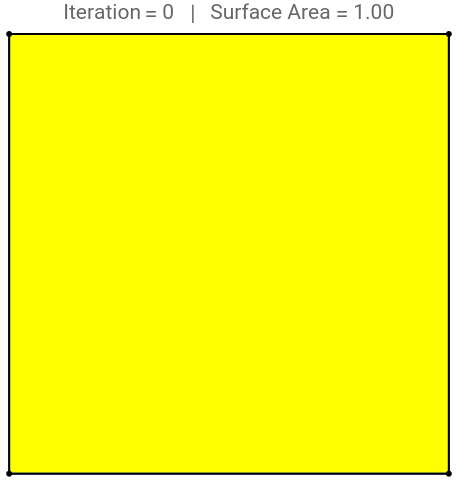
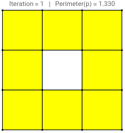
The Menger sponge, discovered by Austrian mathematician Karl Menger in 1926, is originally a 3D fractal that can also be represented in 2D. It’s constructed by repeatedly removing the center one-third of smaller cubes from a larger cube : This process, when repeated infinitely, creates a shape with zero volume same for its 2D version , except that in 2D it creates a shape with zero area.
1. Area of the Menger Sponge (2D) ;
2. Perimeter of the Menger Sponge (2D) ;
2. Perimeter of the Menger Sponge (2D) ;
In[]:=
Table[MengerMesh[n,2,MeshCellStyle->{{1,All}->Red,{0,All}->Black},ImageSize->80],{n,1,4}]
Out[]=
,
,
,
3. Volume of the Menger sponge (3D) ;
4. Surface of the Menger Sponge (3D) ;
5. Fractals measurements.
4. Surface of the Menger Sponge (3D) ;
5. Fractals measurements.
In[]:=
Table[MengerMesh[n,3,MeshCellStyle->{{1,All}->Red,{0,All}->Black},ImageSize->80],{n,1,2}]
Out[]=
 ,

Area of the Menger Sponge (2D)
Area of the Menger Sponge (2D)
In[]:=
a[n_]:=(8/9)^nManipulate[Module[{area,label},area=N[(8/9)^n,3];label=Row[{"Iteration = ",n," | ","Surface Area = ",N[area,{4,5}]}];MeshRegion[MengerMesh[n,2],MeshCellStyle->{{2,All}->Yellow,{1,All}->Black,{0,All}->Black},Boxed->False,PlotLabel->label,ImageSize->230]Plot[a[x],{x,0,20},ImageSize->230,PlotRange->All,Epilog->{Red,PointSize[Large],Point[{n,a[n]}]}]],{n,0,6,1},SaveDefinitions->True]
Out[]=


In[]:=
Limit[a[n],n->∞]
Out[]=
0
Perimeter of the mENGER Sponge (2D)
Perimeter of the mENGER Sponge (2D)
In[]:=
p[n_]:=(4/3)(8/3)^nManipulate[Module[{perim,label},perim=N[p[n],3];label=Row[{"Iteration = ",n+1," | ","Perimeter(p) = ",NumberForm[perim,{4,3}]}];MeshRegion[MengerMesh[n+1,2],MeshCellStyle->{{2,All}->Yellow,{1,All}->Black,{0,All}->Black},Boxed->False,PlotLabel->label,ImageSize->200]Plot[p[x],{x,0,20},ImageSize->200,PlotRange->All,Epilog->{Red,PointSize[Large],Point[{n,p[n]}]}]],{n,0,6,1},SaveDefinitions->True]
Out[]=
In[]:=
Sum[(4/3)(8/3)^n,{n,0,n,1}]
Out[]=
4
5
-1-n
3
3+3n
2
1+n
3
In[]:=
Limit(-),n->∞
4
5
-1-n
3
3+3n
2
1+n
3
Out[]=
∞
Volume of the Menger sponge (3D)
Volume of the Menger sponge (3D)
In[]:=
v[n_]:=(20/27)^nManipulate[Module[{vol,label},vol=N[(20/27)^n,3];label=Row[{"Iteration: ",n," | ","Volume(v)= ",NumberForm[vol,{4,3}]}];MeshRegion[MengerMesh[n,3],MeshCellStyle->{{2,All}->Yellow,{1,All}->Black,{0,All}->Black},Boxed->False,PlotLabel->label,ImageSize->200]Plot[v[x],{x,0,20},ImageSize->200,PlotRange->All,Epilog->{Red,PointSize[Large],Point[{n,v[n]}]}]],{n,0,6,1},SaveDefinitions->True]
Out[]=

In[]:=
Limit[v[n],n->∞]
Out[]=
0
Surface of the Menger Sponge (3D)
Surface of the Menger Sponge (3D)
In[]:=
s[n_]:=2(20/9)^n+4(8/9)^nManipulate[Module[{surf,label},surf=N[2(20/9)^n+4(8/9)^n,3];label=Row[{"Iteration: ",n," | ","Surface(s)= ",NumberForm[surf,{4,3}]}];MeshRegion[MengerMesh[n,3],MeshCellStyle->{{2,All}->Yellow,{1,All}->Black,{0,All}->Black},Boxed->False,PlotLabel->label,ImageSize->200]Plot[s[x],{x,0,20},ImageSize->200,PlotRange->All,Epilog->{Red,PointSize[Large],Point[{n,s[n]}]}]],{n,0,6,1},SaveDefinitions->True]
Out[]=

Fractals measurements (MENGER SPONGE)
Fractals measurements (MENGER SPONGE)
A fractal measure is a way to describe the size or complexity of a fractal shape, even when it doesn't fit traditional geometric rules. It helps quantify how much space a fractal takes up, using tools like fractional dimensions to capture its detailed, self - repeating structure.
2D
2D
Explanation: At each iteration of the 2D version of the Menger sponge, the square is divided into a 3×3 grid (9 smaller squares), and 1 square (the center) is removed, leaving 8 self-similar pieces, each scaled down by a factor of 1/3.
The 2D version of the Menger sponge has a fractal dimension of approximately 1.89, which lies between a line (1D) and a surface (2D). This means it is more complex than a simple curve, but it doesn’t fully cover a 2D area.
3D
3D
Explanation: In 3D, the cube is divided into 27 smaller cubes (3×3×3), and 7 cubes are removed, leaving 20 self-similar cubes, each scaled down by 1/3.
The 3D Menger sponge has a fractal dimension of approximately 2.73, meaning it is more complex than a surface but not quite a full 3D volume.
sIERPINSKI TRIANGLE/Pyramid
sIERPINSKI TRIANGLE/Pyramid
The Sierpinski triangle,invented by Wacław Sierpiński in 1915. is just an other type of fractals similar to the menger sponge , except that it is made of equilateral triangles, each time one fourth of the shape is removed creating 3 smaller equilateral triangles.
1. Area of the Sierpinski Triangle (2D) ;
2. Perimeter of the Sierpinski Triangle (2D) ;
2. Perimeter of the Sierpinski Triangle (2D) ;
3. Volume of the Sierpinski Pyramid (3D) ;
4. Surface of the Sierpinski Pyramid (3D) ;
5. Fractals measurements.
4. Surface of the Sierpinski Pyramid (3D) ;
5. Fractals measurements.
Area of the Sierpinski triangle (2D)
Area of the Sierpinski triangle (2D)
Perimeter of the Sierpinski triangle (2D)
Perimeter of the Sierpinski triangle (2D)
Volume of the Sierpinski Pyramid (3D)
Volume of the Sierpinski Pyramid (3D)
Surface of the Sierpinski Pyramid (3D)
Surface of the Sierpinski Pyramid (3D)
Fractals measurements (Sierpinski triangle/Pyramid)
Fractals measurements (Sierpinski triangle/Pyramid)
2D
2D
Explanation: At each step, the triangle is divided into 4 smaller triangles, but the central triangle is removed, leaving 3 self - similar parts, each scaled down by a factor of 1/2
The Sierpinski triangle has a fractal dimension of approximately 1.58, placing it between a one-dimensional curve and a two-dimensional surface. It is more detailed than a line but does not fully occupy a 2D area, reflecting its infinite emptiness and recursive structure.
3D
3D
Explanation: The 3D version (Sierpinski pyramid/tetrahedron) splits a pyramid/tetrahedron into 8 smaller ones, but 4 are removed, leaving 4 self-similar pieces, each scaled by 1/2.
The Sierpinski pyramid/tetrahedron has a fractal dimension of exactly 2, meaning it behaves like a surface in three-dimensional space. Although it appears as a 3D object, its internal structure lacks volume—it’s a hollow form that mimics the dimensionality of a 2D surface within 3D space.
Koch snowflake
Koch snowflake
The von Koch flake curve is another type of fractal, by Swedish mathematician Helge von Koch in 1904. Constructed by starting with an equilateral triangle and repeatedly replacing the middle third of each line segment with an equilateral triangle pointing outward.
1. Area of the Koch snowflake (2D) ;
2. Perimeter of the Koch snowflake (2D) ;
3. Fractals measurements.
2. Perimeter of the Koch snowflake (2D) ;
3. Fractals measurements.
Area of the Koch snowflake(2D)
Area of the Koch snowflake(2D)
Perimeter of the Koch snowflake (2D)
Perimeter of the Koch snowflake (2D)
Fractals measurements (Koch SnowFLAKE)
Fractals measurements (Koch SnowFLAKE)
2D
2D
At each step of its construction, each line segment is divided into 3 parts, and the middle part is replaced with two sides of an equilateral triangle, creating 4 self-similar segments, each scaled down by 1/3.
The Koch snowflake has a fractal dimension of approximately 1.26, which places it between a straight line (1D) and a surface (2D). It’s more detailed than a simple curve, with infinite length, but it still cannot fully cover an area. Its repeating triangular pattern gives it a complex, jagged structure that never smooths out, no matter how much you zoom in.
Peano curve
Peano curve
The Peano curve is a type of fractal, first described by Italian mathematician Giuseppe Peano in 1890. It was one of the first examples of a space - filling curve, a continuous curve that completely fills a 2D area, such as a square.The curve is constructed by recursively dividing a square into a 3×3 grid of smaller squares, then drawing a path that connects the nine squares in a specific order. At each step, the process is repeated within each smaller square.
Perimeter of the peano curve
Perimeter of the peano curve
Fractals measurements (PEANO CURVE)
Fractals measurements (PEANO CURVE)
2D
2D
The Peano curve is a space-filling curve that, in its limit, passes through every point of a square. At each iteration:
- The square is divided into 9 smaller squares (a 3×3 grid),
- The curve becomes 9 self-similar parts,
- Each scaled down by a factor of 1/3.
- The square is divided into 9 smaller squares (a 3×3 grid),
- The curve becomes 9 self-similar parts,
- Each scaled down by a factor of 1/3.
The Peano curve has a fractal (Hausdorff) dimension of exactly 2, which means it completely fills a two-dimensional area. Even though it is defined as a continuous curve (usually 1D), its recursive construction allows it to behave like a surface. This illustrates how fractals can defy traditional geometric expectations by transforming a line into something that occupies full 2D space.
Conclusion
Conclusion
CITE THIS NOTEBOOK
CITE THIS NOTEBOOK
Understanding fractals through Menger sponge and more
by Yacine Driss
Wolfram Community, STAFF PICKS, August 27, 2025
https://community.wolfram.com/groups/-/m/t/3536402
by Yacine Driss
Wolfram Community, STAFF PICKS, August 27, 2025
https://community.wolfram.com/groups/-/m/t/3536402