ORIGINAL ARTICLE: Shin, Hee-Young, A computational approach to Ricardo’s and Marx’s business cycle models (2022). Available at SSRN: http://dx.doi.org/10.2139/ssrn.4187298
Abstract: One important contribution made by both David Ricardo and Karl Marx is their nonlinear dynamical reasoning for understanding key macroeconomic variables. This note aims to reconstruct some crucial aspects of their nonlinear business cycle theories utilizing the computational power of Wolfram Mathematica. Mathematica enables us to set up, solve, and visualize a system of more than two multivariable differential equations that cannot be solved manually. Utilizing the computational power of this software, we can replicate Ricardo’s and Marx’s nonlinear dynamical model of business cycle and attempts to extend their original baseline model to account for some new stylized facts of contemporary phenomena such as the effect of financialization, of rentiers’ income and of corporate offshoring phenomenon on the business cycle pattern in our economic system.
Keyword: business cycle, predator-prey model, differential equation systems, Wolfram Mathematica.
JEL Classification: B16, C60.
JEL Classification: B16, C60.
Introduction to this note
Introduction to this note
This note is a supplementary notebook for the draft “Revisiting Ricardo's and Marx's business cycle model: A computational approach.”
Both David Ricardo and Karl Marx are one of the greatest classical political economists whose economic theories and models have contributed to our deeper understanding of the dynamics of capitalist market economies. In this article, we revisit both Ricardo and Marx’s core analyses of how the accumulation of capital stock will have an influence on the distribution of relative income among different social classes and how this relative income distribution pattern will affect on the speed and phase of capital accumulation over time.
By nature, Ricardo and Marx’s analyses on this issue is based upon their high level inductive reasoning that involves considerations of cumulative causation among multi-variables. In this article, we attempts to transform their core ideas into a number of systems of multi-variable differential equations and to find and visualize the solution path utilizing the computational power of Wolfram Mathematica.
The article consists of relatively self-contained multiple sections, each section discussing, for example, (1) Ricardo’s and Marx’s original business cycle model (in two separate sections), followed by(2) extending their baseline models to account for the effect of financialization, of corporate offshoring, and of increasing rentier’s income on the accumulation of private domestic industrial capital (in two separate sections).
Following the structure of the article, this notebook introduces some of the functionalities of Wolfram Mathematica used to identify the basic model parameters, the solution, and visualization result discussed in each section of the article.
Ricardo’s rent-profit-wage dynamics
Ricardo’s rent-profit-wage dynamics
Core ideas
Core ideas
Regarding the long-run effect of capital accumulation on differential (ground) rent and (nominal) wages in agricultural sector, Ricardo proposes the idea that capital accumulation in agricultural sector tends to increase both demand for labor and nominal wages on the one hand and in consequence prices of foods and ground rent that capitalist farmers pay to owners of land also tend to rise. This rising differential rent soon becomes an obstacle to a further accumulation of capital because a greater portion of gross profits of capitalist farmers must be paid to landowners. This predator-prey relation between landowners and capitalist farmers becomes more complicated when it instigates the dynamic interaction and interest conflict between capitalists and wage laborers in the same sector.
Variables, parameters, and the model
Variables, parameters, and the model
We can transform Ricardo’s idea into a system of three differential equations. Let x ≡ rT, y ≡ wL, and z ≡ πK. Then we can write this dynamic and interdependent relationships among the three income variables in the following way:
x
y
z
This system consists of three first-order, homogeneous, autonomous, (non-) linear differential equations, which requires some qualitative analyses.
One analytical solution and its simulation
One analytical solution and its simulation
One possible analytical solution to this system can be found by assuming that nominal wages are brought down to their subsistence level, thereby transforming the variable y not any more binding as an independent variable.
In this case, the entire system is reduced to a system of two differential equations that is similar to a classic predator-prey relation between rent and profit income:
x
z
If we assign some arbitrary values to each parameter and set initial values, we can generate the following simulation:
In[]:=
ClearAll[a,c,α,β,γ,x,y,z,t];a=2;α=1.2;c=1.5;γ=1;sol=NDSolve[{x'[t]==-ax[t]+αx[t]z[t],z'[t]cz[t]-γx[t]z[t],x[0]3,z[0]3},{x[t],z[t]},{t,0,30}]
Out[]=
x[t]InterpolatingFunction[t],z[t]InterpolatingFunction[t]


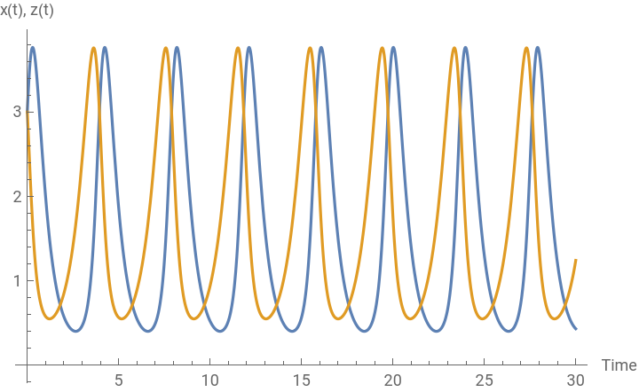
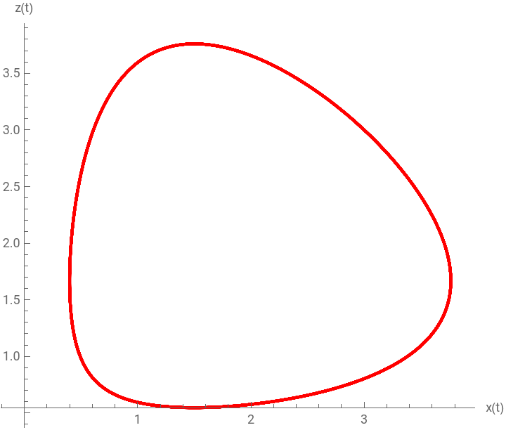
As we can see Figures below, there emerges a clear classic predator-prey relation in between the rent income and profit income over time. As the gross profit for agricultural capitalists increases, agricultural farmers can lease out a greater unit of arable land to cultivate and produce more agricultural products. If this happens, the rent tends to rise over time, ultimately lowering the agricultural profits. As this happens, capital accumulation in the agricultural sector slows down, so does the rent income with a certain time lag. In this nonlinear dynamical relation between the two income variables, the profit for agricultural capitalists plays a role as a prey, while the rent for the owner of land a predator.
In[]:=
Plot[Evaluate[{x[t],z[t]}/.sol],{t,0,30},PlotLegends{"predator","prey"},AxesLabel{"Time","x(t), z(t)"}]
Out[]=


In[]:=
ParametricPlot[Evaluate[{x[t],z[t]}/.sol],{t,0,30},PlotStyle{Red,Thick},AxesLabel{"x(t)","z(t)"}]
Out[]=
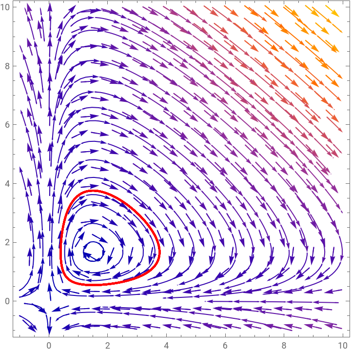
We can also draw a phase diagram in which forces in the vector field defined by the very differential equations in the model is visualized. The following Figure shows how we can visualize a solution curve for the interacting two variables inside the phase diagram.
In[]:=
Manipulate[Show[VectorPlot[{-ax+αxz,cz-γxz},{x,-1,10},{z,-1,10}],StreamPlot[{-ax+αxz,cz-γxz},{x,-1,10},{z,-1,10}],ParametricPlot[Evaluate[{x[t],z[t]}/.sol],{t,0,b},PlotStyle{Red,Thick}]],{b,30,50},SaveDefinitions->True]
Out[]=


Another solution candidate and related simulation
Another solution candidate and related simulation
Another approach to solving this system is to (1) transform the third equation into a second-order differential equation and attempt to find an analytical solution, (2) conduct a qualitative analysis by drawing 3D phase plane, and (3) run a simulation with some arbitrary parameter and initial values.
Given the original system,
x
y
z
The time derivative of yields =c-γx-γz-δz - . This can be rewritten as = (c - γ x -δ y) - (+)z. This is a linear, non-autonomous, second-order differential equation, whose variables coefficients are functions of x and y.
z
..
z
z
z
x
y
δy
z
..
z
z
γ
x
δ
y
Unfortunately, we can not find any analytical solution to this equation because it involves variable coefficients whose values are dependent on the solution to another system of two differential equations. Even if we can find some computational expressions for the solution, it is hardly interpretable. Therefore, we should rely on a phase diagram analysis.
In[]:=
DSolve[z''[t]==(c-γx[t]-δy[t])z'[t]-(γx'[t]+δy'[t]),z[t],t]
Out[]=
z[t]+(1.5-1.x[K[1]]-1.δy[K[1]])K[1]+(1.5-1.x[K[1]]-1.δy[K[1]])K[1](-1.[K[2]]-1.δ[K[2]])K[2]K[3]
2
t
∫
1
K[3]
∫
1
1
K[3]
∫
1
K[3]
∫
1
-(1.5-1.x[K[1]]-1.δy[K[1]])K[1]
K[2]
∫
1
′
x
′
y
For this purpose, let us assign some arbitrary values to parameters and draw the following 3D phase plane:
In[]:=
ClearAll[a,c,α,β,γ,x,y,z,t];a=2;α=1.2;b=1.5;β=1.3;c=1.5;γ=1;δ=1.4;Show[VectorPlot3D[{-ax+αxz,-bx+βyz,cz-γxz-δyz},{x,-10,10},{y,-10,10},{z,-10,10}],StreamPlot3D[{-ax+αxz,-bx+βyz,cz-γxz-δyz},{x,-10,10},{y,-10,10},{z,-10,10}]]
Out[]=

As this 3D plot shows, there is a clearly discernable predator-prey relationship in the domain between rent and profit income. As soon as we introduce a third, inverse wage-profit dynamics, this predator-prey relation turns into a more complex chaotic motion.
This chaotic interaction among the three variables captured in this phase portrait should remind the readers of either the Lorenz equations (Lorenz 1963) or Chemostat models (Herbert and Telling 1956). It is also similar to a food chain model of three interacting species (McLaren and Peterson 1991).
Marx’s profit-wage dynamics
Marx’s profit-wage dynamics
Core ideas
Core ideas
According to Marx, the ground rent no longer plays a crucial role in determining the distribution of national income in his lifetime and in the future. The dynamic relation between profit-investment and wage-employment is pronounced as the rising rents and prices of agricultural product cease to be binding.
Under these circumstances, a new socioeconomic and class dynamics emerged, and it is directly related with the effect of capital accumulation on the demand for labor. A higher rate of profit and the continual capital stock accumulation tends to require a greater demand for labor if the reinvested portion of surplus value proportionately increases both means of production (constant capital) and labor power (variable capital) required for the production of commodities. If this process continues, both the demand for labor and nominal wages will rise. But as soon as nominal wages increase, the profit income and rate of profit tend to fall, thereby slowing down the process of capital accumulation.
Variables, parameters, and the model
Variables, parameters, and the model
Marx’s core idea can be represented by the following system of two differential equations where new variables x ≡ πK and y ≡ wL.
This model consists of two nonlinear, first-order differential equation , for which we can conduct some qualitative analyses.
A simulation for some possible solution paths
A simulation for some possible solution paths
Let us simulate some solution paths of this system of differential equations after assigning arbitrary parameter values and the initial condition as a way to visualize the behavior of solutions near the steady state value. Let α = 2, β = 1.2, γ = 1 and δ = 0.9. Let us also suppose that the initial number of both x and y is also given by x(0) = 3 and y(0) = 3, respectively. The ‘NDSolve’ function in Mathematica allows us to generate a time series of numerical solutions of the two differential equations starting from the initial condition. The syntax for this simulation is as follows:
The simulation result, which is contained in the ‘InterpolatingFunction’ for both variables, x(t) and y(t), can be visualized by the following syntax:
We can also plot the trajectory of interactions between the two variables, treating them as functions of time. For this purpose, we use the ‘ParametricPlot’ function in Mathematica.
As anticipated, two variables constantly move in counterclockwise spelling out an orbital circle centering around the second steady state value of the system. As one variable increases (decreases), another variable also increases (decreases). But as soon as the second variable increases (decreases) the first variable is negatively (inversely) affected.
A simulation with varying parameter values
A simulation with varying parameter values
Alternatively, we can generate an interactive chart that allows us to change the value of each parameter. For this purpose, we use ‘ParametricNDSolve’ function in Mathematica that automatically generates possible numerical solution values for each parameter. With the previously defined initial value, the following syntax computes the values of unknown parameters.
The ‘ParametricFunction’ for each variable contains the simulated values of all four parameters for both x(t) and y(t). We can visualize this parametric function as follow:
The effect of corporate offshoring on domestic employment and labor income
The effect of corporate offshoring on domestic employment and labor income
Some stylized facts
Some stylized facts
One important feature of our contemporary capitalist market economies is unmitigated corporate offshoring practice that has hollowed out the productive sector of domestic economy. As more and more big companies close down their factories and move them in other countries where cost of production is lower than their home countries, both the demand for labor and nominal wages for employed fall. At aggregate level, this myopic corporate offshoring practice has worsened the problems associated with uneven regional economic development and de-industrialization of some parts of domestic economy.
A model specification and the possible solution path I
A model specification and the possible solution path I
One way of accounting for this phenomenon is to include an additional variable that captures the migration of capital stock. If we assume that the corporate offshoring decision is primarily driven by differential labor costs, the rate and volume of external migration of domestic capital can be analyzed by the interaction between domestic profit income share and labor income.
Let us think of the scenario that the profit income share domestically generated is decreasing at a rate proportional to the number of labor income share. As the nominal wage and the demand for labor reach a certain critical point, an increasing number of domestic companies begins to relocate their production facilities into other national territories seeking relatively lower labor cost.
Using this modified equation, we can conduct a series of qualitative analyses as follow:
First, the steady state points of the system of two differential equations can be found by:
Next, let us assign an arbitrary value to each parameter, such as α = 2, β = 1.2, γ = 1, and δ = 0.9. The corresponding interactive solution path with varying values of parameter k becomes:
We can also draw a phase diagram, in which two steady state points and parametric plot are included:
Compared to Marx’s original business cycle model discussed above, the level of respective income share is substantially reduced, and it decreases further as we increase the value of k. The bigger the size of k, which means that the greater number of companies offshore their production facilities, the smaller the domestically produced national income and labor income share. This simulation-based model prediction is consistent with many empirical studies of the effect of corporate offshoring on domestic income distribution and employment
A model specification and the possible solution path II
A model specification and the possible solution path II
With this modification, the system is now having three differential equations as follows:
We can also run a set of multiple simulations with a varying value of ω in the following way:
Compared to the previous model, we have much more volatile and unstable nonlinear dynamical relationship between the two income share components. As before, the level of respective income share is substantially reduced in this formulation. It is also noticeable that domestically generated profit income is swung widely as we increase the size of oscillating parameter value ω (given k). Not only the labor income share is reduced but also the stability of employment and income is disturbed by cyclical factors.
The effect of financialization and increasing rentier’s income on wage share
The effect of financialization and increasing rentier’s income on wage share
Some stylized facts
Some stylized facts
Another important aspect of our contemporary economic systems is associated with the proliferation of various fictitious capitals and the greater dependency of industrial capital on the need of short-term financial portfolio management. Various economic agents have been increasingly dependent on the need of financial portfolio management, and even nonfinancial corporate business firms have shifted their business priority onto short-term financial management rather than focusing on the expansion of real business operations such as the accumulation of fixed investment, R&D, product innovation, and employment.
This financialization of the major sectors of the economy is often coupled with various schemes (both institutions and practices) to privatize and appropriate surplus value to the hands of a few shareholders of technology-based venture capitals and real estate companies. Along the way, even more complex institutionalized systems of income transfer from the productive and industrial sector of capital to unproductive and parasitic sectors of the society have emerged.
Variables, parameters, and the model
Variables, parameters, and the model
This financialization and increasing income transfer to various types of rentiers have substantially modified the traditional capital-labor relation. For our purpose, we may be able to account for these phenomena by introducing a third variable that intervenes and modifies the profit-wage dynamics.
Interestingly, the proto type model of this complex system consisting of more than three variables is that of Ricardo. As we saw earlier, Ricardo's rent-profit-wage dynamic is captured by the following system of three differential equations:
Let us slightly modify Ricardo’s system into the following form:
And further into:
In this successive modification, we retain Ricardo’s original insights and continue assume that x variable is a positive function of y variable. The z variable also increases as it interacts with y variable. The variable y decreases as a result of interaction between x and z. The only difference from Ricardo’s model is that we have simplified the growth of x variable and reduced the number of parameters for simplicity.
In our context, of course, the variables represent something different from Ricardo’s original usage. The variable y represents the growth of industrial capital and profit income accruing to industrial capitalists, while x represents wage laborers whose employment and income depends on its interactions with industrial capitalists. The variable z, in this context, denotes the change in rentier income stemming from either financial management (i.e., various incomes from portfolio management) or real estate management (i.e., various incomes from rental and lease, asset sales, etc).
This modified Ricardo system can show nonlinear dynamical interactions among industrial capital, wage labor, and rentiers. Notice that this reduced form of the system at hand is the same as Lorenz equations.
A simulation for some possible solution paths
A simulation for some possible solution paths
The steady state points of the last system are:
Following the standard procedure, let us arbitrarily assign some values to parameters and initial conditions to identify possible solution paths.
The forces at work surrounding this system can be visualized by the following phase diagram:
This figure retains the same property that we observed in Ricardo’s rent-profit-wage dynamics. The new feature is that, with some unique parameter values, this three-dimensional profit-rentier-wage dynamics can spell out a complex chaotic motion articulated by Lorenz equations. Divestment from the productive sector and an ever-increasing income transfer to nonproductive sector of the economy can make the system extremely fragile and vulnerable to various shocks.
The phase diagram and the simulation with varying parameter values
The phase diagram and the simulation with varying parameter values
We can also create an interactive chart that shows the dynamic behavior of the system with varying parameter values.
A programming for interactive simulations
A programming for interactive simulations
For the purpose of running multiple simulations with varying parameter value, we can write the following syntaxes:
Concluding remarks
Concluding remarks
In this note, we have introduced a number of powerful Wolfram Mathematica functionalities that are used in the article “Revisiting Ricardo’s and Marx’s business cycle model: A computational approach.”
The article itself aims to reconstruct both Ricardo’s and Marx’s business cycle models and to evaluate their contemporary relevance, especially in the face of new stylized facts of the economy such as financialization, corporate offshoring, and the increasing concentration of rentier income.
Some useful functionalities of Wolfram Mathematica has enabled us to easily identify the model structure and parameters, to find and visualize the solution path that cannot be attained by hands. The author appreciates any useful comments and suggestions for improving the current manuscript.
CITE THIS NOTEBOOK
CITE THIS NOTEBOOK
A computational approach to Ricardo's and Marx's business cycle models
by Hee-Young Shin
Wolfram Community, STAFF PICKS, August 17, 2023
https://community.wolfram.com/groups/-/m/t/2992791
by Hee-Young Shin
Wolfram Community, STAFF PICKS, August 17, 2023
https://community.wolfram.com/groups/-/m/t/2992791