Radiolarians are marine amoebas that grow silica shells which become siliceous oozes once they die. Spumellaria are a subspecies of radiolarians that grow intricate patterned shells with radial symmetry using biochemical mechanisms. There is little to no information about the growth process of Spumellaria, and this project aims to model their development computationally and draw conclusions as to why they grow in the patterns they do. My theory discusses potential causes for locations of spine growth along with the intracellular stages that prompt spine growth on the radiolarian species.
Introduction
Introduction
Radiolarians are unicellular marine organisms that have exceptionally intricate exoskeletons constructed from silica despite their miniscule size. In their life cycles they absorb silica compounds from their marine environment that forms the hard inorganic frame of their skeleton. When Radiolarians die and sink to the bottom of the ocean they constitute siliceous oozes which are the rarest forms of deep sea biogenic pelagic sediments, only covering about 15% of the ocean floor (Mulder, 2011).
Divided into four major subclasses, each radiolarian has an individual skeletal structure and is taxonomically classified on the basis of extruding mineral depositions. The subclasses include Acantharea, Nassellaria, Spumellaria and Phaeodaria, each of which exhibit morphologically differing characteristics.
This project computationally models the process of radiolarian exoskeleton growth, focussing on the subclass of Spumellaria. It’s the only species of Radiolarian that has radial symmetry, making it an ideal subject to study through mathematical models. Its exoskeleton is contained in its ectoplasm, and grows in approximately symmetrically spaced out spines/spicules of silica. The process of its exoskeletal growth is known as silicification, and results in an average of 12-15 spine growths per Spumellaria. It is nearly impossible to study the growth of Radiolarians in the laboratory since they cannot be kept alive in simulated environments, which means that there is a minimal understanding of its morphological and biochemical development processes.
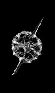
This is what a Spumellaria looks like through an electron micrograph, with irregularly spaced pores on the skeleton as well as spines on the shell . The Spumellaria is currently in the first stages of growth, hence it has only 2 spines .
Biochemical Approach
Biochemical Approach
To be able to depict the growth of the skeleton, the machinations of the growth must be better understood, which includes the organism’s motive for growing the skeleton as well as the process by which it grows this skeleton. Due to a lack of authentic research there is little concrete evidence of biochemical skeletal formation, but it is generally accepted that it does so through the process of bio-mineralization. The primary component of bio-mineralization in Spumellaria is silicic acid or H2O3Si, which is formed from orthosilicic acid monomers or Si(OH)4 dissolved in the seawater around them. This indicates that the dehydration of the silica compound forms the solid silica depositions on the surface. Transporter proteins carry the silicic acid to vesicles, and as the concentrations reach a maximum threshold, the polymerization process begins.
This code defines each of the molecules as combinations of Silicon, Hydrogen & Oxygen, so that they can be used to represent actual molecules later in the process:
In[]:=
orthosilicicAcid=Molecule[{Atom["Si","Silicon"],Atom["O","Oxygen"],Atom["O","Oxygen"],Atom["O","Oxygen"],Atom["O","Oxygen"],Atom["H","Hydrogen"],Atom["H","Hydrogen"],Atom["H","Hydrogen"],Atom["H","Hydrogen"]},{Bond[{1,2},"Single"],Bond[{1,3},"Single"],Bond[{1,4},"Single"],Bond[{1,5},"Single"],Bond[{2,6},"Single"],Bond[{3,7},"Single"],Bond[{4,8},"Single"],Bond[{5,9},"Single"]}];silicicAcid=Molecule[{Atom["Si","Silicon"],Atom["O","Oxygen"],Atom["O","Oxygen"],Atom["O","Oxygen"],Atom["H","Hydrogen"],Atom["H","Hydrogen"]},{Bond[{1,2},"Single"],Bond[{1,3},"Single"],Bond[{1,4},"Double"],Bond[{3,5},"Single"],Bond[{2,6},"Single"]}];silicon=Molecule[{Atom["Si","Silicon"],Atom["O","Oxygen"],Atom["O","Oxygen"]},{Bond[{1,2},"Double"],Bond[{1,3},"Double"]}];
In[]:=
silicicAcid=Molecule[{Atom["Si","Silicon"],Atom["O","Oxygen"],Atom["O","Oxygen"],Atom["O","Oxygen"],Atom["H","Hydrogen"],Atom["H","Hydrogen"]},{Bond[{1,2},"Single"],Bond[{1,3},"Single"],Bond[{1,4},"Double"],Bond[{3,5},"Single"],Bond[{2,6},"Single"]}];
In[]:=
silica=Molecule[{Atom["Si","Silicon"],Atom["O","Oxygen"],Atom["O","Oxygen"],Atom["O","Oxygen"],Atom["O","Oxygen"]},{Bond[{1,2},"Single"],Bond[{1,3},"Single"],Bond[{1,4},"Single"],Bond[{1,5},"Single"]}];
In[]:=
GraphicsRow[{MoleculePlot[orthosilicicAcid],"=",MoleculePlot["Water",ImageSize->150],"+",MoleculePlot[silicicAcid]}]
Out[]=
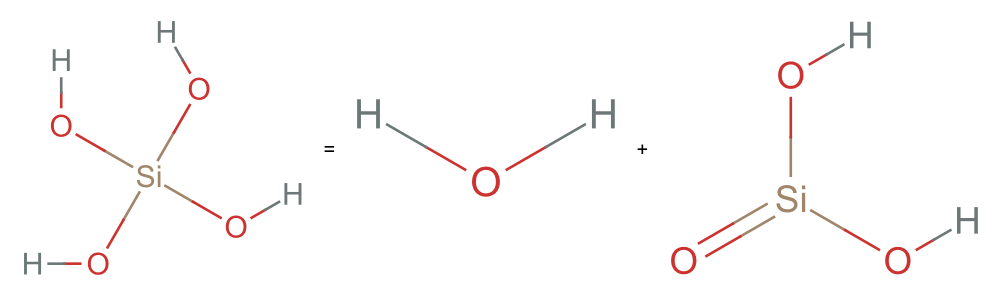
When the silicic acid reaches maximum concentration within the vesicle, it is further dehydrated into SiO2 which forms a giant molecular network that is deposited in a spicular pattern upon the surface of the Radiolarians latticed exoskeleton.
In[]:=
GraphicsRow[{MoleculePlot[silicicAcid],"=",MoleculePlot["Water",ImageSize->150],"+",MoleculePlot[silicon]}]
Out[]=
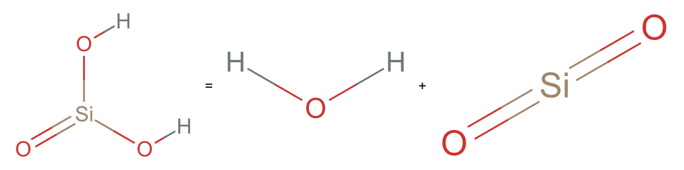
Effectively, the orthosilicic acid is absorbed, dehydrated twice to create silicon dioxide by the radiolarian. The water is released from the cell through exocytosis, and vacuoles are filled with air to make the organism more buoyant.
The code below orders the chemicals in order of their compounds within the radiolarian:
In[]:=
GraphicsRow[{MoleculePlot[orthosilicicAcid],MoleculePlot3D[orthosilicicAcid,ImageSize->Small],"->",MoleculePlot[silicicAcid],MoleculePlot3D[silicicAcid,ImageSize->Small],"->",MoleculePlot[silicon],MoleculePlot3D[silicon,ImageSize->Small]}]
Out[]=
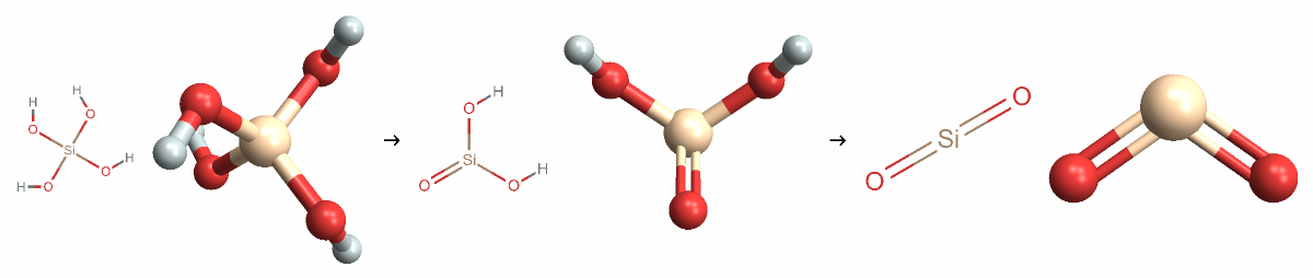
The orthosilicic acid is carried into Silica Deposition Vesicles (SDV’s) by Silica Transporter Proteins (SIT’s) which are coded for genetically. The family of proteins was first discovered in diatoms, and speculated to exist in Radiolarians as well. SIT’s are sodium-coupled active transport proteins that perform specific silica uptake functions within eukaryotes (Marron, 2016). This acid is then dehydrated to produce silicic acid, which is then accumulated within the vesicles until the vesicle reaches a maximum concentration as monitored by the SITs.
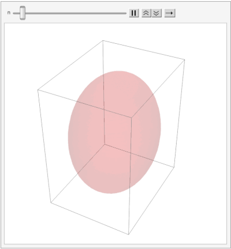
The code below animates an ellipsoid to change it’s colour opacity as a symbol for the absorption of silicic acid, and reaches a maximum threshold at the highest opacity:
In[]:=
AnimatedImage[Import[NotebookDirectory[]<>"Vesicle.gif"]]
Out[]=
From the information available, and various renderings of the exoskeleton it can be surmised that the radiolarian uses it for a myriad of purposes, including but not limited to:
◼
Protection
◼
Balance & Buoyancy
◼
Maximising Surface Area
Theory
Theory
My theory focuses on explaining the cycles of spine growth using the concentration of silicic acid as the regulating factor. The SDVs are intracellular components right under the surface of the ectoplasm that produce the bio silicified valves. I visualise them to be spaced out evenly with each vesicle absorbing orthosilicic acid from the seawater they are exposed to – allowing them to uptake silica simultaneously but at different rates depending on the silica concentration in the environment around them.
According to me, each of the vesicles begin absorbing silica at roughly the same time, when the organism starts building its exoskeleton. The difference in the availability of silica in their environments determines which vesicle reaches maximum concentration first.
The first vesicle to reach maximum concentration begins growing the first spine on the radiolarian. It requires energy for this process which it derives from adenosine triphosphate (ATP) molecules that are produced from aerobic respiration. I think that the vesicle that reaches maximum concentration first depletes the ATP produced, and uses all the silicic acid available nearby – rendering it impossible for adjacent vesicles to generate the next spike.
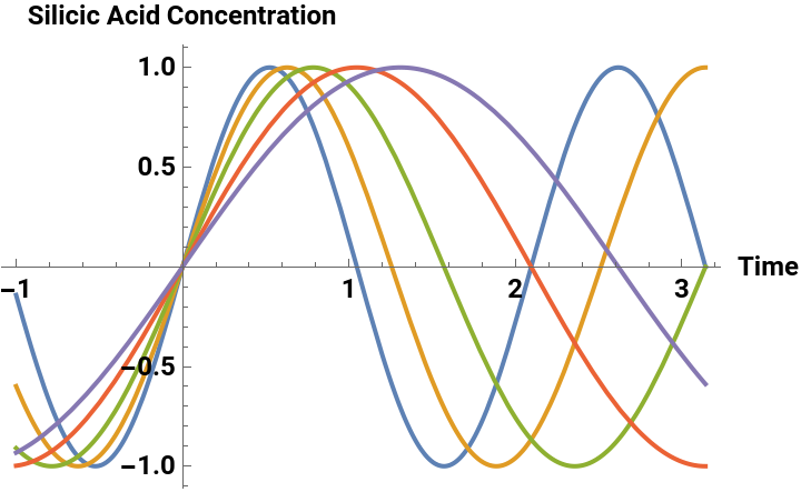
In this way spine growth is ordered. An exclusion zone, which is the result of silicic acid distribution & usage, is determined, which decides where the next spines cannot grow. Barring these vesicles, the next vesicle to reach maximum concentration is the one to grow the next spike. I also believe that the spikes are grown in order to keep the organism afloat within the water, so the exclusion zone is an explicitly growth restrictive zone, but the next spike is most likely to grow as far away as possible from the previous one. The graph below uses arbitrary units to plot the change in concentration of silicic acid within 5 different vesicles over a period of time since there is no actual data to determine what the maximum concentration of silicic acid is.
Plotting a graph using a sine function to model vesicle concentration peaks:
In[]:=
Plot[{Sin[3x],Sin[2.5x],Sin[2x],Sin[1.5x],Sin[1.2x]},{x,-1,Pi},PlotLegends->{"Vesicle 1","Vesicle 2","Vesicle 3","Vesicle 4","Vesicle 5"},AxesLabel->{"Time","Silicic Acid Concentration"},LabelStyle->Directive[Bold, Black,Medium]]
Out[]=


The specific average of between 12-15 spines on each Spumellaria suggests the presence of a gene that codes for a certain number of spines before the exoskeleton is grown. This would more accurately explain the radially symmetrical distribution of each of the spines, since the organism would know where to grow them for them to be relatively equally spaced out. The Lsi2 & Lsi genes code for the SIT proteins that monitor silicic acid concentration & are responsible for its transportation as well. An adjacent gene that codes for spine growth rate and number would be logically progressive and also explain the ability of the organism to grow spines in a way that it balances itself within the water. Spumellaria, like most other radiolarian species, are nonmotile, which means that they must maximise their buoyancy to float in the water.
There are a myriad of possible reasons for the symmetrical distribution of spine growth which include balance in currents, buoyancy and maximising surface area to feed from. The spherical nature of the organism makes it naturally buoyant in water, but the addition of spines in sequential growth would need to be evenly distributed to prevent it from being weighed down by the silica. The extension of these spines also allow food particles to get stuck onto the spikes, resulting in pseudopodia from within the cell reaching out to pick it up and feed on it. The fact that the spines stick out as extensions of the organism increase the surface area from which it can grab its food. Furthermore, the hard and spiky nature of the spines offer a layer of protection to the otherwise vulnerable ameboid.
Bi-dimensional Representation
Bi-dimensional Representation
Spumellaria growth can be modelled using two dimensional silicification patterns to understand the origins of silica deposition on its exoskeleton. The actual structure of the Spumellaria contains layers of silica, and maps a network of pores and spicula or spines (Anderson, 1998) which constitutes it’s exoskeleton. Since the organism is spherical in shape, it can be reduced to a circular diagram to be represented two dimensionally. The Spumellaria grow between 12-15 spines on average, depending on their size, so when reducing the dimensions, the number of spines growing is reduced to ~6 spines. First, the directionality of each of the spines is determined, by splitting the circle into 6 equal angular segments showcasing how the spines grow outwards. The arrows render the emergence of each spine from the surface of the Spumellaria.
Animation using circle points to generate arrows in position of spines:
In[]:=
Animate[Graphics[Arrow[{{0,0},#}]&/@CirclePoints[x],PlotRange->{{-1,1},{-1,1}}],{x,0,7},SaveDefinitions->True,AnimationRunning->False]
Then I visualised the placement of each spine, when there are different numbers of spines on the radiolarian starting with 1 spine, all the way up to 6 spines. The 2D diagrams create an even split using divisions of 2π around the circle. This creates the base of where each spine is located on my 2D Spumellaria.
Graphics & Graphics Row to order each location of spine origin on a 2D circle:
However, my aim is to visualise the growth of these spines, so an animation needed to be rendered that depicts these spines moving around the skeleton, showcasing the appearance of more than one. First, a function that converts polar coordinates to Cartesian coordinates must be defined in order to return an integer list of points around the circle that would create symmetry between the total number of points present on the circle.
Function to convert polar coordinates to Cartesian coordinates:
This creates an “Exclusion Angle” which is the arc of the circle near an existing point determining where no other point can appear.
Defined function to generate coordinates of points on a circle that will be evenly spaced out from another:
Using a manipulate function, the list of coordinates generated by this function can be seen as the exclusion angle increases from 3π/2 to π/3.
The list of coordinates represents the number of points on the circle at a given exclusion angle. For example at 3π/2, there is one singular set of coordinates representing one singular point on the circle.
The circle points function was then entered into graphics and animated to produce a visual that showcases the movement of points around the circle as in when the exclusion angle changes from 3π/2 to π/3:
3-Dimensional Modelling
3-Dimensional Modelling
After the two dimensional representation, the idea of exclusion angles and equally spaced points are easier to understand, so when the dimensions are increased the foundational concept of points on a shape can be retained. In 3-dimensions the organism can be modelled as a sphere, so I first tried to decide where each spine would be located if there were between 1 to 15 spines.
These were ordered in a row:
I then decided to use these points as origin points for spines – which I want to use cones to model. The cone function requires the input of start and end coordinates along with the radius. I used ToSpherePoints & FromSpherePoints functions to convert each of the points into equally spaced out points on the sphere. I then increased the height uniformly for each sphere, and gave them an arbitrary radius of 0.05.
I used the graphics function to render all of them as 3D images of the cones. The graphics row created shows all the cones angled differently based on their start and end coordinates:
However, I realised that the built in FromSpherePoints function had issues when certain coordinates were entered, which I encountered when I tried to render it with more than 10 cones at a time. I entered parameters using if statements that decided what occurs when the return functions would not be possible. For example when sphere points are re-converted from points {0,0, coordinate}, computing the ArcTan value for 0 is impossible since it’s undefined.
To subvert this I entered parameters into this function that would prevent it from crashing when certain coordinates are entered:
Made a cone converter function which generates a cone using the coordinates and height entered, which can be mapped onto the sphere points function to create multiple equally spaced out cones protruding from the surface of the sphere:
Mapping this function onto a range of sphere points using Graphics3D generates a set of cones that are equally spaced out on the surface of a, currently invisible, sphere of radius 1:
This is done by making coneConv a pure anonymous function that uses SpherePoints coordinates as it’s origin input and returns cones of height 1.5 units. The function without the Graphics3D returns cone functions with the coordinates and radius, giving the locations of each of the cones instead of the visuals.
Wrapped in Graphics3D to produce visual:
A separate function using the same premise as coneConv, generates coordinates for cylinders that are equally spaced out on the surface of the sphere:
Unlike the cones however, these cylinders will extend from the centre to the surface of the circle, projecting circular “holes” that represent the porous exoskeleton.
The next function combines the two functions above to generate a 3D graphic of the radiolarian with a porous exoskeleton, and the number of cones entered as an input:
This creates a master function that generates a model which grows spines and becomes porous simultaneously.
Stored as frames within:
The function was animated to generate a visual that progresses sequentially:
However this model runs on the assumption that all spines grow simultaneously, which is not what my theory posits. In my theory I suggest that each vesicle that reaches maximum silicic acid concentration begins silica deposition on the surface of the cell. In my next model, I use a function that changes the height of the spine and the opacity of my vesicle, to model the process of growth of a single spine on the surface of the radiolarian’s exoskeleton.
I developed two different functions that generate cone height and vesicle opacity as functions of time:
Piecewise functions were used to decide the rate of change for each parameter on the basis of time:
I also generated a cone radius function that changes the radius alongside the height:
This function combines the three functions above to generate a visual of the layers of the cell during spine growth:
It changes the radius of the spine during growth, predicting that the silica deposition happens in upward spirals instead of a pyramid style building.
Stored within:
Animated to generate moving visual:
However this model is not compatible with my theory since I use the premise that there is an organic matrix that codes for the location and size of each spine before it starts growing. In the version compatible with my theory, the organic matrix pre-decides the radius of the cone, and grows it vertically instead of vertically and horizontally.
In this function, I combined the two height and opacity functions into a larger function that generates a stacked version of these graphics:
This showcases the layers of the exoskeleton all the way down to the vesicle, and shows a front view of what it would look like for an individual spine to grow.
The function was mapped to a range of t = 15, incremented at 0.1 frames to generate a list of frames:
The following code then animated those frames to progress rapidly like a short video clip:
When they first start growing, their amoeba itself is growing as the cytoplasm separates into the endoplasm & the ectoplasm. At this point in time, according to me, they collect silica uniformly across their membrane, forming a thin shell of spherical silica. However, the cell needs to be able to reach food, and at this point the silica shell is thin enough for pseudopodia from the cell to reach out. The silica layer is still nascent and the pseudopodia can easily break through – forming the small pores that exist in its exoskeleton. For this reason the porous nature of the exoskeleton must serve a functional purpose allowing the cell to reach food. The first phase of the following model showcases the growth of the organism as the sphere slowly expands.
Then as soon as the cell is as big as it gets, the silica starts depositing in the pattern of rings – around the holes that are formed by the pseudopodia extending into the water around them. This solidifies the circular holes on the first layer of their skeleton. The radial symmetry of this shell maximises the surface area from which they can reach food in the environment permitting the pseudopodia to get the greatest amount of food from the sea. The second phase of the model shows this formation of pores in the shell of silica as a function of time – as time increases so does the density of pores.
Once they have a feeding mechanism in place, they also need protection from predators. Since they’re extremely small, and their porous exoskeleton would allow other organisms to easily reach the cell, they would need more effective protection from being eaten. This causes the deposition of subsequently acquired silicic acid in the form of spines on the exoskeleton. There is evidence of an organic matrix within the radiolarian (Afanasieva, 2014) which pre-decides the location of each spine growth, supporting the theory that silicification is gene controlled. The concentration controlled vesicle mechanism is the reason that the spines grow far apart from one another – when a vesicle uses its concentrated silicic acid, it requires energy to do so, draining the capability for an adjacent vesicle to produce a subsequent spine. I then wanted to extrapolate the above code, and apply it to a larger graphic which produces individual spines in succession.
The functions below model sphere radius growth, number of points on the sphere and spine number with respect to time, in t units:
This function repeats a list of values at regular intervals of five to control the growth of individual spines:
These were plotted to showcase the change over time, since they would all overlap:
A function to model the number of spines and their individual heights at a particular time was created:
I then used a function to generate random starting points for the spine grow function so that every time the animation is generated, there’s a new starting point and the spines don’t all grow next to each other:
I then wrote a rotate function that codes for the angle of rotation to change at a particular rate. Since I knew that the total time was 100 units, I wanted the viewpoint to rotate once around the entire model, meaning that it would need to complete a 2Pi rotation in 100t. I wrote a function that could serve as an argument for the angle in the larger Rotate function in the master function:
All of these time functions were combined into a master function that represented the process of radiolarian growth completely using graphics directives to render 3D images:
The master function was mapped onto a range of points t, from 1 to 100 at increments of 0.5. These became frames, summing to 200 frames stored in the variable final frames.
A video generate function was used to play the final frames as a rapid movie that lasted 15 seconds:
This video is a potential growth model for Spumellaria that is in alignment with my theory for their growth patterns. It starts with an expanding sphere, which is representative of the amoeba itself, and then as pseudopodia begin to reach out to grab food silica deposits in rings around them. This creates the porous skeleton on which the spines start to grow one by one.
Conclusion
Conclusion
From these progressive visualisations it can be understood that Spumellaria grow in clear stages starting with a general silica shell, developing pores in their exoskeleton and finally building spines that form patterns. The radial symmetry of this growth suggests underlying functionalities that control the generation of each spine. My theory suggests possible reasons for the symmetry and order of the spinal growth, as well as the mechanisms by which the radiolarian silicifies.
My model combines three major growth phases as classified by me:
◼
Shell formation: The growth of the amoeba as a general layer of silica is deposited – creating a uniform outer silica shell
◼
Porous lattice: The gradual creation of holes on the skeleton as in when the pseudopodia reach out to grab food from the marine environment. The general deposition of silica in rings as the holes become more and more prominent, spreading uniformly across the surface to maximise the area from which the radiolarian can reach its food.
◼
Spine Growth: Once the porous skeleton is formed, the radiolarian starts growing spines across its surface as a means for protection, balance and increasing surface area for food absorption. The spines grow in a random order, with no two spines growing adjacent to each other in succession. This signifies the “exclusion zone” that is created by the vesicles using energy to dehydrate silicic acid concentrations into hard silica deposits.
Through the course of this project I learned to apply functional programming in order to render graphics, which make them flexible, easy to edit and more subject to custom changes. As a whole, this project was a computational & biological endeavour to explain the behaviour of a certain organism that used code to communicate my theories and ideas as visuals.
Future Works
Future Works
Currently only one species of Radiolarians was looked at, and in the future I would like to examine the silicification patterns for non-radially symmetrical radiolarian exoskeletons. Many different species develop conical exoskeletons or irregular polygons, and I want to understand and model why these species differ in their morphology. Additionally this current model could be improved upon by including a more clear visual of the organic matrix that codes for the silicification locations as well as the transport proteins that are responsible for the movement of silica within the organism. Since the model applies my theory of silicification it achieves the purpose of explaining how the spines grow, but in the future I would like to create a more sophisticated visual representation for the same idea.
Acknowledgements
Acknowledgements
I would like to thank Stephen Wolfram & the program directors for establishing the framework for my computational essay and helping me decide the direction in which I want to take my research. I would like to extend my gratitude to my mentor David DeBrota for consistently answering my questions and helping me work through problems with my research. Without him this project would not be possible. Finally, I would like to thank my peers Tony Song & Annie Zhu for providing suggestions and peer reviews to refine and edit my paper making it the version that it is.
Bibliography
Bibliography
◼
Common Minerals in Biomineralization. (2017, February 11). Time Scavengers. https://timescavengers.wpcomstaging.com/introductory-material/generalscience/common-minerals/
◼
Demetrio Boltovskoy, Anderson, O. R., & Correa, N. (2017). Radiolaria and Phaeodaria. 731–763. https://doi.org/10.1007/978-3-319-28149-0_19
◼
Estroff, L. A. (2008). Introduction: Biomineralization. Chemical Reviews, 108(11), 4329–4331. https://doi.org/10.1021/cr8004789
◼
Heintze, C., Pötschke, P., Pohl, D., Jannes Hauptstein, Bernd Rellinghaus, & Kroeger, N. (2020). An intimate view into the silica deposition vesicles of diatoms. BMC, 2(1). https://doi.org/10.1186/s42833-020-00017-8
◼
Hori, R. S., Shinki, T., Iwakiri, A., Matsuoka, A., Suzuki, N., Ogane, K., & Tuji, A. (2021). Growth pattern of the siliceous skeletons of living Spumellaria (Radiolaria) from the Kuroshio Current, offshore southwestern Shikoku Island, Japan. Revue de Micropaléontologie, 71, 100504. https://doi.org/10.1016/j.revmic.2021.100504
◼
How can an organosilcon lifeform break down silicates. (n.d.). Worldbuilding Stack Exchange. Retrieved July 11, 2024, from https://worldbuilding.stackexchange.com/questions/192571/how-can-an-organosilcon-lifeform-break-down-silicates
◼
HyperBook, B. (2024, June 17). Unveiling the Chemistry of Radiolaria: Exploring Elemental Insights and Environmental Significance. Bioengineering Hyperbook. https://bioengineering.hyperbook.mcgill.ca/unveiling-the-chemistry-of-radiolaria-exploring-elemental-insights-and-environmental-significance/
◼
Kaoru Ogane, Akihiro Tuji, Suzuki, N., Matsuoka, A., Kurihara, T., & Hori, R. S. (2010). Direct observation of the skeletal growth patterns of polycystine radiolarians using a fluorescent marker. Marine Micropaleontology, 77(3-4), 137–144. https://doi.org/10.1016/j.marmicro.2010.08.005
◼
Lazarus, D. B., Kotrc, B., Wulf, G., & Schmidt, D. N. (2009). Radiolarians decreased silicification as an evolutionary response to reduced Cenozoic ocean silica availability. Proceedings of the National Academy of Sciences, 106(23), 9333–9338. https://doi.org/10.1073/pnas.0812979106
◼
Marron, A. O., Ratcliffe, S., Wheeler, G. L., Goldstein, R. E., King, N., Not, F., de Vargas, C., & Richter, D. J. (2016). The Evolution of Silicon Transport in Eukaryotes. Molecular Biology and Evolution, 33(12), 3226–3248. https://doi.org/10.1093/molbev/msw209
◼
Micscape Microscopy and Microscope Magazine. (n.d.). Www.microscopy-Uk.org.uk. http://www.microscopy-uk.org.uk/mag/indexmag.html?http://www.microscopy-uk.org.uk/mag/artfeb05/cbdiatoms.html
◼
Mitani-Ueno, N., Yamaji, N., Huang, S., Yoshioka, Y., Miyaji, T., & Ma, J. F. (2023). A silicon transporter gene required for healthy growth of rice on land. Nature Communications, 14(1), 6522. https://doi.org/10.1038/s41467-023-42180-y
◼
Molecular Expressions Photo Gallery: Radiolarians. (n.d.). Micro.magnet.fsu.edu. https://micro.magnet.fsu.edu/micro/gallery/radiolarians/radiolarians.html
◼
Morphology of the Radiolaria. (n.d.). Ucmp.berkeley.edu. Retrieved July 11, 2024, from https://ucmp.berkeley.edu/protista/radiolaria/radmm.html#:~:text=Varying%20slightly%20from%20one%20subclass
◼
Mulder, T., Hüneke, H., & Van Loon, A. J. (2011, January 1). Chapter 1 - Progress in Deep-Sea Sedimentology (H. HüNeke & T. Mulder, Eds.). ScienceDirect; Elsevier. https://www.sciencedirect.com/science/article/abs/pii/B9780444530004000019?via%3Dihub
◼
Radiolaria: microworld’s architecture. (2009, July 14). MORPHOCODE. https://morphocode.com/radiolaria-microworld-architecture/
◼
Sahebi, M., Hanafi, M. M., Rafii, M. Y., Azizi, P., Abiri, R., Kalhori, N., & Atabaki, N. (2017). Screening and Expression of a Silicon Transporter Gene(Lsi1)in Wild-Type Indica Rice Cultivars. BioMed Research International, 2017, 1–13. https://doi.org/10.1155/2017/9064129
◼
Sandín, M., & Méndez, M. (2019). Diversity and Evolution of Nassellaria and Spumellaria (Radiolaria). https://theses.hal.science/tel-03137926/file/MENDEZ_SANDIN_Miguel_2019.pdf
◼
University~ora@ldeo.columbia.edu, O. R. A.-D. E. O. of C., & Oceanography~smgupta@csnio.ren.nic.in, S. M. G. I. of. (1998, January 28). Evidence of Binary Division in Mature Central Capsules of a Collosphaerid Colonial Radiolarians: Implications for Shell Ontogenetic Patterns in Modern and Fossil Species. Palaeontologia Electronica. https://palaeo-electronica.org/content/1-1-shell-ontogeny-in-radiolarians#:~:text=The%20data%20presented%20here%20suggest
CITE THIS NOTEBOOK
CITE THIS NOTEBOOK
Predicting radiolarian growth patterns through 3D modelling
by Shivika Gupta
Wolfram Community, STAFF PICKS, July 11, 2024
https://community.wolfram.com/groups/-/m/t/3216505
by Shivika Gupta
Wolfram Community, STAFF PICKS, July 11, 2024
https://community.wolfram.com/groups/-/m/t/3216505