CITE THIS NOTEBOOK: Results of the contest "Best Private Investor" from MOEX by Kirill Belov. Wolfram Community OCT 26 2022.
About the contest
About the contest
Every year, from September to December, the Moscow Exchange (MOEX) holds a contest for the "Best Private Investor". Anyone can take part in the competition. Next, I’ll just quote the description from the information page:
The contest “The Best Private Investor 2021” is held by PJSC Moscow Exchange.
The main purpose of the Contest is to demonstrate the opportunities available to private investors when trading instruments of the stock, derivatives and currency markets, as well as the profitability that can be obtained with proper work on these sites. Open publication of transactions and results of the participants of the Contest allows you to quickly monitor the progress of the Contest and the strategies being implemented.
The main purpose of the Contest is to demonstrate the opportunities available to private investors when trading instruments of the stock, derivatives and currency markets, as well as the profitability that can be obtained with proper work on these sites. Open publication of transactions and results of the participants of the Contest allows you to quickly monitor the progress of the Contest and the strategies being implemented.
In this article, we will try to study investor returns using the Wolfram language as a tool for analysis.
I want to emphasize that the main goal of this article is to show readers how the Wolfram language can be used to work with various data. In this case, tables with the results of the competition of the Moscow Exchange were used, but anything could have been instead this results. I used this sattistics because the statistics provided by the Moscow Exchange are magnificent. I was not yet seen a single exchange that would share such good and clear data on how traders trade.
I do not call for investment and trading. Everyone who wants to become a trader must carefully weigh all the risks and most importantly never use more money than he is ready to lose.
Init
Init
First, as is customary in Wolfram, we clear the current context, reduce the size of the calculation history and set the working directory:
In[]:=
ClearAll["`*"]; $HistoryLength = 1; SetDirectory[NotebookDirectory[]];
These steps are optional, but relieve some problems if the user has to work for a long time without restarting the session.
Getting data
Getting data
All contest results in the form of CSV-tables are located at the following address: ftp://ftp.moex.com/pub/info/stats_contest/2021/. This network directory has many nested directories that contain participants’ deals sorted by date, one main directory ftp://ftp.moex.com/pub/info/stats_contest/2021/all/, in which there are generally all transactions of all participants within the framework of the competition and several files with aggregated results:
◼
nomlist.csv - winners
◼
result_day.csv - results on the last day of the competition
◼
trader.csv - list of participants
In this article, we only need a file with the final results. Download it to the working directory:
In[]:=
URLDownload["ftp://ftp.moex.com/pub/info/stats_contest/2021/result_day.csv", "result_day.csv"]
Out[]=
File
Data import
Data import
We will store all the competition data in one variable, which we will call like this:
In[]:=
data = <||>;
Now you need to import the downloaded files, remove the excess and convert the table to a more convenient form for Wolfram:
In[]:=
data["all"] = Normal @ QueryAll, <| "trader" -> "nik", "broker" -> "diler_name", "type" -> "contype_name", "amount" -> "amount" /* (#/61.2&), "volume" -> "vol_rub" /* (#/61.2&), "deals" -> "qty", "profit" -> "dohod_rub" /* (#/61.2&), "activity" -> "uchastnik_activ" |> @ Select[Length[#] == 16&] @ ImportString[#, "Dataset", HeaderLines -> 1]& @ StringReplace[#, ";" -> ","]& @ Import["result_day.csv", "Text", CharacterEncoding -> "WindowsCyrillic"] /. "Срочный" -> "Futures", "Валютный" -> "Forex", "Фондовый" -> "Stock" ; Dataset[data["all"]]
Out[]=


In this table, extra columns have been removed and, for convenience, only the names of the participants have been left (id removed). Also I translated exchange types and converted RUB amounts and volumes to USD with rate 1USD == 61.2RUB on 27.10.2022.
Results
Results
Let’s get to the statistics. First, let’s just see how many unique participants there were without taking into account the type of market:
In[]:=
Length @ DeleteDuplicatesBy[#trader&] @ data["all"]
Out[]=
26053
The ratio of active and inactive unique members:
In[]:=
Block{chartData = Map[Length] @ GroupBy[#["activity"]&] @ DeleteDuplicatesBy[#trader&] @ data["all"]}, PieChartchartData, ChartLabels StringTemplate["Inactive: <*chartData[[1]]*> (<*100*chartData[[1]]/Total[chartData]*>%)"][], StringTemplate["Active: <*chartData[[2]]*> (<*100*chartData[[2]]/Total[chartData]*>%)"][]
Out[]=
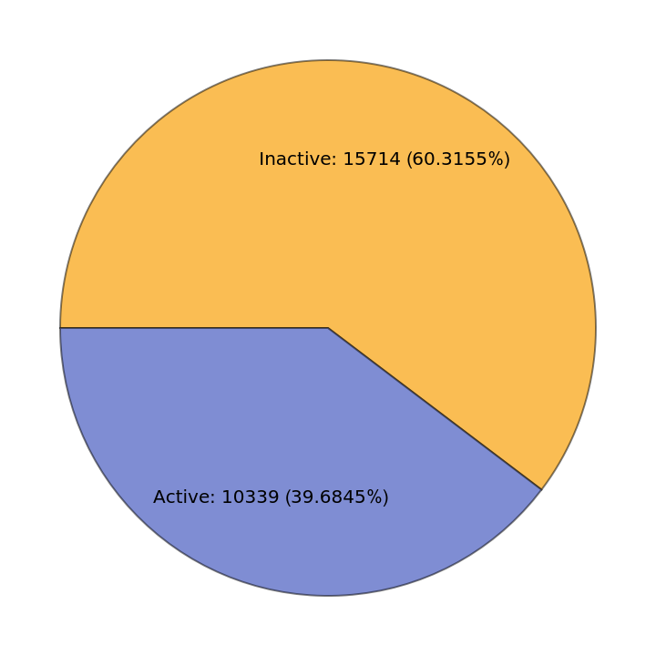
Now let’s look at the ratios for selected types of markets among active participants:
o get a more accurate result, we will consider different types of accounts separately. Obviously, trading in the stock market and in the foreign exchange market will always be very different and mixed will greatly affect the final statistics. Let’s separate these data from the general table for convenience. Plus, we will select only active participants whose starting capital is more than 100,000RUB == 1,633.99:
Why are traders with starting capital less than $1,634 (100,000RUB) not considered? Everything is very simple. In the final results, the Moscow Exchange normalizes all participants by $1,634 if their starting capital was less. Therefore, we cannot know exactly the size of the starting capital of such traders. Therefore, in order not to spoil the statistics with inaccurate data, we do not consider them yet. In any case, the table above shows the largest group of participants, which will give us the most realistic results. After all, in this way we selected an average trader - a professional who invested more than $1,634 in the competition and traded on the stock market.
Let’s make a table for the total, median and average values of starting capital:
The numbers above are misleading, except for the last two lines. The fact is that in statistics, the start-up capital is common for all three accounts, so the total start-up capital can be estimated only for aggregated results - it is about $106.8 million (6.5 billion rubles) for active participants and $148.6 million (9 billion rubles) for all. How many of them were used for a particular type of account is already much more difficult to calculate.
The result for the average value is already more interesting. Here it becomes clearly visible what a big advantage in their favor is created by a lot of inactive traders and traders with a starting capital of less than $1634. For conditionally “professionals”, which we have identified above, the average starting capital is more than $18,700 (1.1 million rubles). Whereas, taking into account inaccurate data, it is reduced by almost three times - to 350 thousand rubles. At the same time, if we knew the exact amounts less than $1,634, the average value would be even lower.
It is also interesting to look at the distribution of start-up capital among the participants. Let’s build a histogram:
Now let’s make the same table for the trading volume and next to it the same number of deals:
In the original data, the volume of trades and the number of transactions are indicated separately for each market. Therefore, in this table, it will have the correct meaning for all rows. Again, you can clearly see how much the trading volume of active participants differs from the average volume for all. By the way, we can always calculate how many participants have zero trading volume:
And now the most interesting, the total and average returns for each group of traders:
Let us first comment on the quite expected results. The average “income” for all active participants in the competition is $1,678. This is about 9% loss, given that the average start-up capital was about $18,800. And to be more precise:
The average income by groups unexpectedly turned out to be higher, but this is all due to the fact that in the groups that were identified by market type there are many traders with zero income specifically on this market, but with non-zero income on others, and again they shift the average values closer to zero . The most indicative is the total loss of active traders, which is $9.53 million.
And now let’s move on to profitability in the foreign exchange market. There, the total earnings amounted to more than $323,5 thousand and the average income was more than $368. Let’s study in more detail the table with currency accounts. First, sort it in descending order of income, and then in descending order of starting capital:
On the first lines of both tables is the same trader M01, who has a starting capital of about $3.93 million and the final income is about $318.4 thousand. Of course, this is quite a possible case, but it is anomalous for our averaged calculations. Let’s see what is the total and average income in the foreign exchange market without taking into account the first line:
Excluding this anomalous case, the yield on the foreign exchange market became about 0.03%. Most likely, there are similar cases in other markets, which strongly stand out from the results of average traders. But we will not consider them, since the total losses are much larger and it is already more difficult to influence them.
The same conclusions can be drawn from the histogram built based on the results of the final income (zero income is not taken into account):
The histograms above clearly show that there is a fairly large group of participants for the stock and derivatives markets, which has income from -$1,500 to $500, but most of the participants still suffered losses and are in the negative part. On the histogram for the currency market, it turned out that there is a very large group that earned from -$100 to $150 rubles. At the same time, the majority is still on the right side, which cannot but rejoice.
As shown above, the total percentage return for all active members is approximately -8.9%. But we are also interested in the number of traders who, following the results of the competition, had a profit or loss. This does not speak about the amounts used on the exchange in trading, but about how successfully each individual trader used trading strategies. Therefore, we first calculate the percentage return for each trader, and then find the average and median values.
Everything looks a little better here. That is, for active participants, the total loss is about 7.7%, and the median loss is about 8.3%. But besides that, let’s also look at the histogram with the percentage distribution of income by participants:
This picture already shows better that much more than half of the participants suffered losses, and quite large ones - many lost up to 50% of their starting capital.
But that’s not all. In addition to the fact that the organizers of the competition decided to ration the majority of participants, there is another problem. All results are given without broker commission, i.e. The Moscow Exchange collected data on transactions only on its side, and the commission was paid outside the exchange. This means that the indicated yield does not take into account how much the trader ultimately paid his broker for working with the exchange. Let’s see which is the most popular broker used by the participants:
The first three places are occupied by Tinkoff, VTB and Otkritie. A short search showed that the basic commissions for the first three brokers are:
We will assume that the default commission for all brokers is the average between 0.04 and 0.05 . To calculate the real “profit” of traders, it is necessary to multiply their trading volume by the broker’s commission and subtract from the final income. Let’s do this, and then build a table and a histogram as it was already done above:
As a result, the losses of active traders actually amount to approximately $24,7 million against $9.5 million without commission. Those. it turns out that brokers earned more than $15 million during this competition alone. Perhaps the prize for the first place should have been given to the Tinkoff bank. Well, let’s also look at the final distribution and percentage yield for each participant:
And distribution:
And the final chart, on which we mark those who earned more/less than 0, more/less than 5%, and more/less than 10%, more/less than 15%:
The following graph shows the distribution of the percentage of participants with income above a certain percentage. For example, according to the chart below you can understand that only a little more than 20% of participants earned more than 0, only 10% of participants earned more than 10%, but about 40% of participants lost more than 20%. In general, this curve can be interpreted as a function of the probability distribution. It shows how much income trader can receive income in the range from -100% to 100% on the x-axis (for a specific chart), if you randomly select any point from in the range (0, 100) on the y-axis:
As a result, this graph can be converted into a function similar to probability density. Only it will not be very smooth, but at the same time suspiciously similar to a normal distribution. And most importantly, the hypothetical peak of this normal distribution will fall on the region from -20% to 0%:
Conclusion
Conclusion
The data that was studied in this article is very good and gives a huge scope for imagination, and the Wolfram language makes it quite easy to visualize all these fantasies in the form of tables, graphs and interactive objects (I couldn’t think of what can be done interactive for this article). I hope that the readers was interested in this little study. Perhaps there are errors and inaccuracies in the article - be sure to report them, and if someone has questions and suggestions - write in the comments or in private messages. Thank you all for your attention!