ABSTRACT (original thesis): This thesis is devoted to the numerical approximation of mechanical systems involving the interaction of a deformable thin-walled structure with an internal or surrounding incompressible fluid flow. In the first part, we introduce two new classes of explicit coupling schemes using fitted meshes. The methods proposed combine a certain Robin-consistency in the system with (i) a projection-based time-marching in the fluid or (ii) second-order time-stepping in both the fluid and the solid. The stability properties of the methods are analyzed within representative linear settings. This part includes also a comprehensive numerical study in which state-of-the-art coupling schemes (including some of the methods proposed herein) are compared and validated against the results of an experimental benchmark. In the second part, we consider unfitted mesh formulations. The spatial discretization in this case is based on variants of Nitsche’s method with cut elements. We present two new classes of splitting schemes which exploit the aforementioned interface Robin-consistency in the unfitted framework. The semi-implicit or explicit nature of the splitting in time is dictated by the order in which the spatial and time discretizations are performed. In the case of the coupling with immersed structures, weak and strong discontinuities across the interface are allowed for the velocity and pressure, respectively. Stability and error estimates are provided within a linear setting. A series of numerical tests illustrates the performance of the different methods proposed. CITATION (original thesis): Mikel Landajuela Larma. Coupling schemes and unfitted mesh methods for fluid-structure interaction. Numerical Analysis [math.NA]. Université Pierre et Marie Curie - Paris VI, 2016. English. ⟨NNT : 2016PA066053⟩. ⟨tel-01366696⟩
This notebook implements a fluid–structure interaction (FSI) solver in pure Wolfram Language. The fluid is governed by the Stokes equations in a 2D rectangular channel, and the structure is a 1D elastic Koiter shell on the top boundary. The coupling uses a semi-implicit kinematically coupled scheme that is unconditionally stable for the added-mass effect – a classical challenge in hemodynamics and aeroelasticity.
Keywords:
fluid–structure interaction, Stokes equations, elastic shell, finite elements, P1/P1, Brezzi–Pitkäranta stabilization, kinematic coupling
fluid–structure interaction, Stokes equations, elastic shell, finite elements, P1/P1, Brezzi–Pitkäranta stabilization, kinematic coupling
1. Problem Description
1. Problem Description
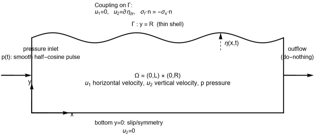
We consider an incompressible Stokes fluid in a rectangular domain Ω = (0, L) × (0, R) coupled to a thin elastic shell on the top boundary Γ = {y = R}. A pressure pulse is applied at the inlet (left boundary), driving a wave that propagates along the compliant wall – a simplified model of arterial hemodynamics.
1.1 Governing Equations
1.1 Governing Equations
The fluid velocity u = (u1, u2) and pressure p satisfy the Stokes equations:
ρf ∂u/∂t - div(2μ ε(u)) + ∇p = 0
div(u) = 0
where ε(u) = (∇u + ∇u^)/2 is the symmetric strain rate tensor.
The thin shell displacement η on Γ satisfies:
ρs ϵ ∂^2η/∂t^2 + c0 η - c1 ∂^2η/∂x^2 = f(t)
where c0 = Eϵ/(R^2(1-ν^2)) is the membrane stiffness, c1 = Eϵ/(2(1+ν)) is the shear stiffness, and clamped endpoints η(0) = η(L) = 0.
The forcing f(t) is the normal fluid stress acting on the shell, i.e. the jump in the normal component of the Cauchy stress tensor across the interface:
f = -( -p I + 2μ ε(u) ) · n · n on Γ
where n is the outward unit normal to Γ (pointing into the structure). For our flat interface n = (0, 1), this simplifies to:
f = p - 2μ ∂u2/∂y on y = R
In the variational (weak) formulation, f does not appear explicitly – it is absorbed into the interface integral when the fluid and solid weak forms are added together.
1.2 Coupling and Boundary Conditions
1.2 Coupling and Boundary Conditions
The fluid and structure are coupled through two conditions on Γ:
Kinematic coupling (continuity of velocity):
u = (∂η/∂t) n on Γ
For our geometry with n = (0,1) this gives u1 = 0 and u2 = ∂η/∂t on the top wall. The fluid velocity must match the shell velocity at every point on the interface.
Dynamic coupling (balance of forces):
σf · n = -σs · n on Γ
where σf = -p I + 2με(u) is the fluid Cauchy stress and σs represents the shell restoring forces (membrane + bending). In the weak form, the fluid stress integral on Γ becomes the shell forcing: the pressure and viscous traction drive the shell motion.
In the semi-implicit kinematic coupling scheme, these are treated as:
• The kinematic condition is enforced implicitly via a Robin BC on the fluid: the u2 equation on Γ includes the shell inertia term (ρs ϵ/Δt) as a penalty-like mass, making the scheme unconditionally stable for the added-mass effect.
• The dynamic condition is enforced by adding the solid stiffness operator (c0 M + c1 K) to the LHS and its contribution from the old displacement to the RHS.
• The shell velocity from the previous time step (woSolid) is fed back as the Robin data on the RHS.
Boundary conditions:
• Bottom (y = 0): Symmetry/slip – u2 = 0
• Top (y = R): Interface – u1 = 0, kinematic coupling for u2
• Left (x = 0): Pressure inlet – smooth half-cosine pulse
• Right (x = L): Do-nothing (natural) outflow
1.3 Numerical Scheme
1.3 Numerical Scheme
We use P1/P1 finite elements with Brezzi–Pitkäranta pressure stabilization for the fluid, and P1 finite elements for the 1D shell. Time integration uses backward Euler with a kinematically coupled splitting: the shell velocity from the previous time step is used as a Robin boundary condition for the current fluid solve. This avoids the added-mass instability that plagues explicit partitioned schemes.
The variational form for the viscous term is: a(u,v) = 2μ ∫ ε(u):ε(v) dΩFor the (u1, u1) block, this expands to: K11 = μ ∫ (2 ∂Na/∂x · ∂Nb/∂x + ∂Na/∂y · ∂Nb/∂y) dΩThe factor 2 on the ∂/∂x term comes from ε11, while the ∂/∂y term comes from 2ε12ε12 with coefficient 2 × (1/2) × (1/2) = 1/2 .
2. Parameters and Setup
2. Parameters and Setup
In[]:=
h = 0.05;dt = 1.*^-4;coef = 20; (* visualization scaling *)lDom = 6.0;rDom = 0.5;eps = 0.1;tFinal = 1.5*^-2;rhos = 1.1;rhof = 1.0;mu = 0.035;nu = 0.5;eY = 0.75*^6;c0 = eY*eps/((rDom^2)*(1 - nu^2));c1 = eY*eps/(2*(1 + nu));nx = Round[lDom/h];ny = Round[rDom/h];tau = 1.0/dt;tau2 = tau*tau;nStep = Round[tFinal/dt];press0 = 2.0*^4;tStar = 0.005;gammap = 0.0001;
Physical parameters: ρf = 1, μ = 0.035, E = 7.5×10^5, ϵ = 0.1 (shell thickness), ν = 0.5 (incompressible shell). The pressure pulse has amplitude P0 = 2×10^4 with duration t* = 0.005.
3. Structured Mesh Generation
3. Structured Mesh Generation
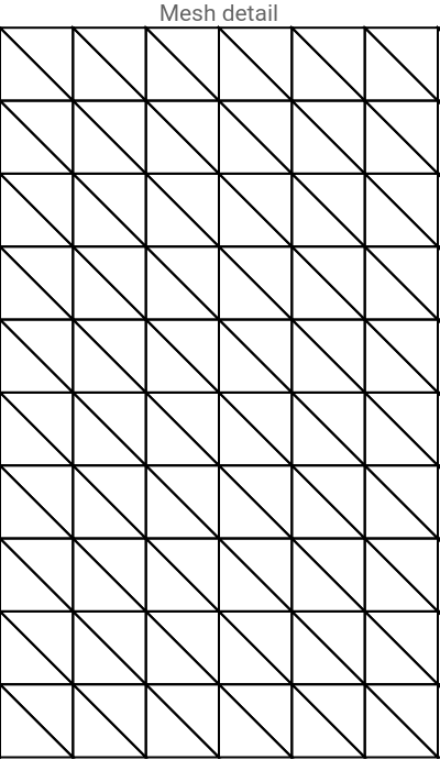
We build a structured triangular mesh. Each rectangular cell is split into two triangles along the same diagonal. This gives (nx+1)(ny+1) = 1331 nodes and 2*nx*ny = 2400 triangles.
In[]:=
Needs["NDSolve`FEM`"];coordsList = Flatten[ Table[{i*lDom/nx, j*rDom/ny}, {j, 0, ny}, {i, 0, nx}], 1] // N;nodeIdx[i_, j_] := j*(nx + 1) + i + 1;triList = Flatten[Table[ Module[{n1, n2, n3, n4}, n1 = nodeIdx[i, j]; n2 = nodeIdx[i + 1, j]; n3 = nodeIdx[i + 1, j + 1]; n4 = nodeIdx[i, j + 1]; {{n1, n2, n4}, {n2, n3, n4}} ], {j, 0, ny - 1}, {i, 0, nx - 1}], 2];fluidMesh = ToElementMesh[ "Coordinates" -> coordsList, "MeshElements" -> {TriangleElement[triList]}];coords = fluidMesh["Coordinates"];nNodes = Length[coords];elements = fluidMesh["MeshElements"][[1, 1]];nElements = Length[elements];Print["Nodes: ", nNodes, " Elements: ", nElements]
Nodes: 1331 Elements: 2400
Visualize the mesh (zoomed in):
ShowfluidMesh["Wireframe"],
Out[]=
4. Boundary and Interface Identification
4. Boundary and Interface Identification
In[]:=
interfaceNodeIndices = Select[Range[nNodes], Abs[coords[[#, 2]] - rDom] < 1*^-10 &];interfaceNodeIndices = SortBy[interfaceNodeIndices, coords[[#, 1]] &];nbint = Length[interfaceNodeIndices];xc = coords[[interfaceNodeIndices, 1]];yc = coords[[interfaceNodeIndices, 2]];bottomNodes = Select[Range[nNodes], Abs[coords[[#, 2]]] < 1*^-10 &];topNodes = interfaceNodeIndices;leftNodes = Select[Range[nNodes], Abs[coords[[#, 1]]] < 1*^-10 &];rightNodes = Select[Range[nNodes], Abs[coords[[#, 1]] - lDom] < 1*^-10 &];ndim = nbint - 2;Print["Interface: ", nbint, " Bottom: ", Length[bottomNodes], " Left: ", Length[leftNodes], " Right: ", Length[rightNodes]]
5. 1D Shell Finite Element Matrices
5. 1D Shell Finite Element Matrices
The shell displacement is discretized with P1 elements on the interior interface nodes (excluding the clamped endpoints). The 1D mass and stiffness matrices are tridiagonal.
6. Fluid Finite Element Assembly
6. Fluid Finite Element Assembly
We assemble the full 3N×3N Stokes system matrix. DOF ordering is [u1, u2, p] with each block of size N. The element loop computes viscous stiffness, mass, pressure–velocity coupling, and Brezzi–Pitkäranta pressure stabilization.
Build the sparse matrix, summing any duplicate entries:
7. Interface Coupling and Boundary Conditions
7. Interface Coupling and Boundary Conditions
8. RHS Mass Matrix and Factorization
8. RHS Mass Matrix and Factorization
9. Time Integration Loop
9. Time Integration Loop
At each time step we: (1) Assemble the RHS from the old solution, the pressure load, the solid velocity feedback, and the solid stiffness. (2) Solve the linear system using the pre-factorized matrix. (3) Update the solid displacement and velocity.
10. Visualization
10. Visualization
10.1 Pressure Field at Final Time
10.1 Pressure Field at Final Time
10.2 Interface Displacement Evolution
10.2 Interface Displacement Evolution
10.3 Interactive Animation
10.3 Interactive Animation
10.4 Average Inlet Pressure Over Time
10.4 Average Inlet Pressure Over Time
10.5 Animated Pressure Field and Interface Displacement
10.5 Animated Pressure Field and Interface Displacement
11. Summary and Implementation Notes
11. Summary and Implementation Notes
What this notebook demonstrates:
• A complete from-scratch P1/P1 Stokes finite element solver in Wolfram Language
• 1D Koiter shell finite elements for the structure
• Kinematically coupled FSI time-stepping (unconditionally stable for the added-mass effect)
• Brezzi–Pitkäranta pressure stabilization for equal-order elements
• Structured mesh generation
• Dirichlet BCs via the penalty method
• 1D Koiter shell finite elements for the structure
• Kinematically coupled FSI time-stepping (unconditionally stable for the added-mass effect)
• Brezzi–Pitkäranta pressure stabilization for equal-order elements
• Structured mesh generation
• Dirichlet BCs via the penalty method
CITE THIS NOTEBOOK
CITE THIS NOTEBOOK
Finite element implementation of kinematically coupled Stokes–shell fluid-structure interaction
by Mikel Landajuela
Wolfram Community, STAFF PICKS, February 13, 2026
https://community.wolfram.com/groups/-/m/t/3639911
by Mikel Landajuela
Wolfram Community, STAFF PICKS, February 13, 2026
https://community.wolfram.com/groups/-/m/t/3639911