This notebook explores key concepts in qubit physics through numerical simulations based on circuit QED parameters. It progressively moves from simplified qubit-only models to the full Jaynes–Cummings Hamiltonian, enabling the study of a wide range of physical phenomena. This approach allows us to probe the interplay between the qubit and resonator, and to investigate effects that go beyond simplified approximations.
Install and load the Wolfram Quantum Framework paclet:
In[]:=
PacletInstall["https://www.wolfr.am/DevWQCF",ForceVersionInstall->True]
Out[]=
PacletObject

In[]:=
<<Wolfram`QuantumFramework`<<Wolfram`QuantumFramework`SecondQuantization`
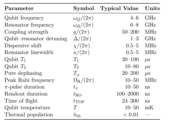
Parameters reference values for transmon-based QED circuits, the following simulations will use values from this table:
Pulses and waveforms
Pulses and waveforms
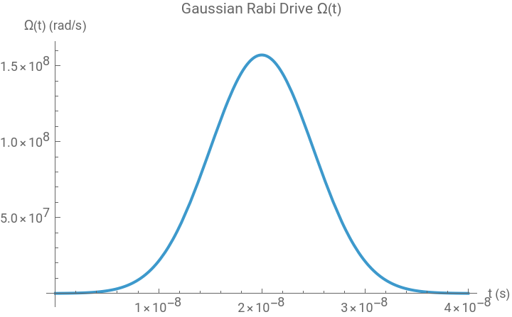
Square and gaussian pulses are widely used in qubit physics because they provide a practical balance between simplicity and physical accuracy in both control and readout
Define a gaussian pulse:
In[]:=
GaussianPulse[RefMax_,t0_,sigma_]:=Function[t,RefMax*Exp[-(t-t0)^2/(2sigma^2)]]
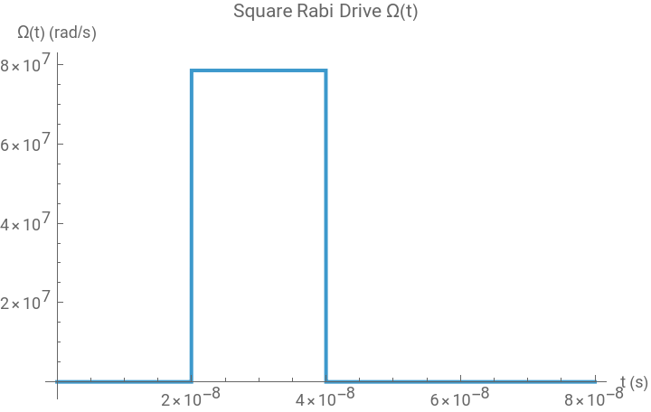
Define a square pulse:
In[]:=
SquarePulse[Ω0_,{ti_,tf_}]:=Function[t,Piecewise[{{Ω0,ti<=t<=tf}},0]]
Plot a gaussian pulse drive with a time-scale of 20 ns:
In[]:=
With{τ=20*^-9},PlotGaussianPulse[π/τ,τ,τ/4][t],{t,0,2τ},
Out[]=
Plot a square pulse of duration 20 ns, that does not start on the time origin:
In[]:=
With{τ=40*^-9},PlotSquarePulse[Pi/τ,{τ/2,τ}][t],{t,0,2τ},
Out[]=
Simulation of qubit only
Simulation of qubit only
A first approach of approximation is modelling only the qubit. The qubit is a transmon qubit with states (|0〉, |1〉) that has a transition frequency 2π approximately between 4-6 GHz. The Hamiltonian using the rotating frame on resonance for the qubit is:
ω
Q
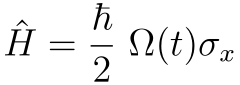
where Ω(t) is a drive envelope, since the resonator is traced out there is no readout dynamics
Let’s see examples of phenomena that can be described using this approach
Time Rabi with square pulse
Time Rabi with square pulse
Set a control parameter related to pulse duration:
In[]:=
τ=40*^-9;
Define a Hamiltonian on resonance (rotating frame) with a square pulse that does not start on the time origin:
In[]:=
H=QuantumOperatorSquarePulseΩmax,τ.8,τ.[t]"X","Parameters"->Ωmax,τ.;
1
2
Evolved state:
In[]:=
evolved=QuantumEvolve[H[8Pi/τ,τ],QuantumState["0"],{t,0,2τ}];
Extract the probability of finding the qubit in the |1〉 state:
In[]:=
prob1=evolved["Probability"][|1〉];
Rabi oscillations during the pulse:
In[]:=
Plotprob1,{t,0,τ},
Out[]=
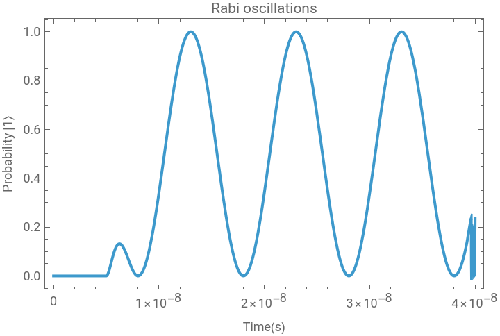
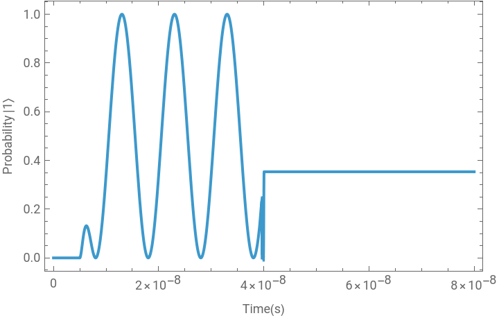
And show what happens after the pulse:
In[]:=
Plotprob1,{t,0,2τ},
Out[]=
Two π/2 pulses
Two π/2 pulses
Define Ω(t) as a sequence of two square pulses with a free interaction part also of duration τ:
In[]:=
H=QuantumOperator"X","Parameters"->Ωmax,τ.;
SquarePulseΩmax,0,τ.[t]+SquarePulseΩmax,2τ.,3τ.[t]
2
Pulse duration:
In[]:=
τ=40*^-9;
Use the Hamiltonian with π/2 pulses and use QuantumEvolve to get the differential equation:
In[]:=
diffEq=QuantumEvolve[H[π/2/τ,τ],QuantumState["0"],{t,0,3τ},"ReturnEquations"->True]
Out[]=
[t]SparseArray.s.[t],s.[0]SparseArray,s.,t,0,
′
s.


3
25000000
Solve for the state vector as function of time:
In[]:=
sol=s./.NDSolve[Sequence@@Normal/@diffEq,Method->"ExplicitRungeKutta",MaxStepSize->τ/30][[1]];
Plot the probability:
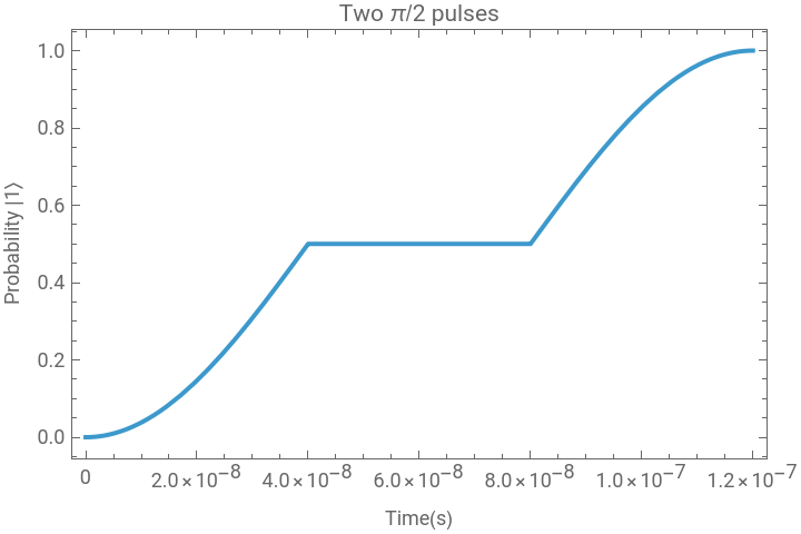
In[]:=
Plot,{t,0,3τ},
2
Abs[sol[t][[2]]]
Out[]=
Gaussian Pulse with varying width
Gaussian Pulse with varying width
Control parameter:
Define the Hamiltonian that uses a gaussian pulse:
Vary the width of the gaussian pulse and plot the scaled pulse and the probability:
Power Rabi
Power Rabi
It is also possible to observe oscillations varying the strength of the driving field
Time scale parameter:
Define Ω(t) with a square pulse :
Extract the probabilities at the final time:
Evolve the |1〉 state:
Extract the probability:
Plot the probability:
Square pulse with decoherence
Square pulse with decoherence
Set up the Hamiltonian:
Include decoherence effects:
Parameter values:
Evolve the state and compute the probability:
Given the parameters and time window, slow loss of amplitude of oscillations:
Full Jaynes-Cummings (Rotating Frame)
Full Jaynes-Cummings (Rotating Frame)
Rotating frame Hamiltonian:
Square Envelopes (no decoherence)
Square Envelopes (no decoherence)
Qubit Hamiltonian:
Resonator Hamiltonian:
Coupling Hamiltonian:
Square pulses (readout after the initial drive):
Full Hamiltonian:
Parameters values:
Evolution of the state:
Sample I-Q values during readout for qubit states |0〉,|1〉 and |+〉:
Compute the IQ values varying the amplitude of the coherent state |α〉
Gaussian drive pulse in qubit + decoherence
Gaussian drive pulse in qubit + decoherence
Lindblad operator related to photon loss, where κ is the resonator linewidth:
Define the photon loss decay channel:
Hamiltonian definition, now we use a gaussian pulse for the initial drive and a square pulse for the readout:
Define the associated Lindbladian:
Set up the values of the parameters:
Initial state |g〉〈g| ⊗ |2〉〈2|:
Perform evolution until the time the readout pulse ends:
Plot also the mean number of photons in the cavity:
Show the IQ values for this case:
References
References
◼
Qubit Physics and Simulation, Theory & Implementation Notes, QUALink Paclet — Bridging Waveform Simulation to Physics Prediction,
February 2026
February 2026
◼
◼
Transmon: a system for superconducting quantum computers
https://community.wolfram.com/groups/-/m/t/3526952
https://community.wolfram.com/groups/-/m/t/3526952
CITE THIS NOTEBOOK
CITE THIS NOTEBOOK
Numerical exploration of qubit–resonator physics in cQED
by Bruno Tenorio
Wolfram Community, STAFF PICKS, March 20, 2026
https://community.wolfram.com/groups/-/m/t/3666521
by Bruno Tenorio
Wolfram Community, STAFF PICKS, March 20, 2026
https://community.wolfram.com/groups/-/m/t/3666521