CGE of Producer Gas in Co-Gasification of Two Biomasses (Mathematica vs. Aspen-Plus)
Asma Hammami, Housam Binous, Hatem Dhaouadi and Ahmed Bellagi
CGE of Producer Gas in Co-Gasification of Two Biomasses (Mathematica vs. Aspen-Plus)
Asma Hammami, Housam Binous, Hatem Dhaouadi and Ahmed Bellagi
Asma Hammami, Housam Binous, Hatem Dhaouadi and Ahmed Bellagi
We consider olive pomace + grape pomace gasification (or biomass co-gasification) in the presence of oxygen only.
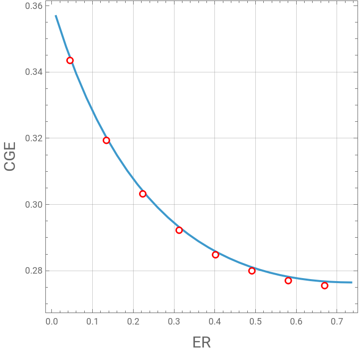
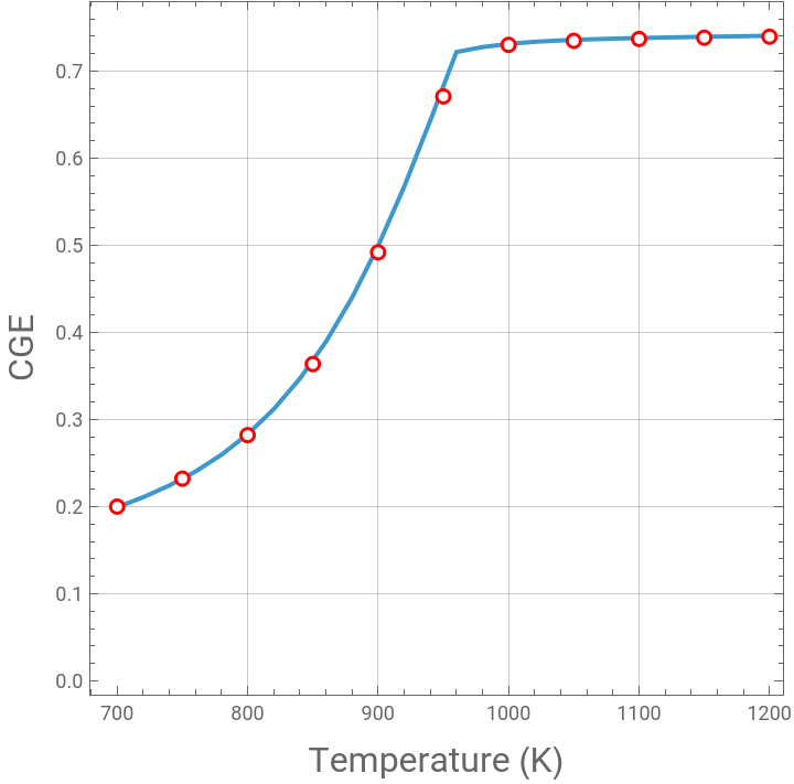
We investigate (1) the effect of temperature and (2) Equivalence Ratio (ER) on the Cold Gas Efficiency (CGE) of the process.
Based on proximate and ultimate analyses, given in Aspen-Plus, olive pomace is modeled as a pseudo-compound whose formula is while grape pomace is modeled as .
CGE calculated using Mathematica agree closely with their counterpart given by Aspen-Plus.
We investigate (1) the effect of temperature and (2) Equivalence Ratio (ER) on the Cold Gas Efficiency (CGE) of the process.
Based on proximate and ultimate analyses, given in Aspen-Plus, olive pomace is modeled as a pseudo-compound whose formula is
C
1
H
1.53015
O
0.501421
C
1
H
1.30934
O
0.438956
CGE calculated using Mathematica agree closely with their counterpart given by Aspen-Plus.
In[]:=
In[]:=
sol[{x_,ER_}]:=Quiet@FindMinimum[{Re[Gtot[x,P]],{n[7]<1/1000000,n[1]>0,n[2]>0,n[3]>0,n[4]>0,n[5]>0,n[6]>0,n[7]>0,n[8]>0,n[9]>0,n[10]>0},n[1]+n[5]+n[4]+n[10]1+1,4n[1]+2n[2]+2n[3]1.53015+1.30934,n[3]+n[4]+2n[5]+n[6]+2n[7]+2n[9]0.501421+0.438956+2ER2.2397,n[6]+n[7]+2n[8]0.0},Table[{n[j],0.07},{j,1,10}],MaxIterations10000,AccuracyGoal5];(*xistemperatureandERisequivalenceratio*)
In[]:=
P=1;
Temperature effect on CGE for ER=0.446
BIOMASS 1 :
C
1
H
1.53015
O
0.501421
In[]:=
(*Defineatomicweights*)atomicWeights=<|"C"->12.01,"H"->1.008,"O"->16.00,"N"->14.01|>;(*Definecompoundformula(subscriptscanbedecimal)*)compound=<|"C"->1,"H"->1.53015,"O"->0.501421,"N"->0.0|>;(*Step1:Molecularweight*)molecularWeight1=Total[compound[#]*atomicWeights[#]&/@Keys[compound]];Print["Molecular weight (g/mol) = ",molecularWeight1];(*Step2:Massfractions*)massFractions=AssociationMap[compound[#]*atomicWeights[#]/molecularWeight1&,Keys[compound]];(*Step3:LHVperkgusingDulongformula*)LHVperKgB1=100(0.3391*massFractions["C"]+1.4444*massFractions["H"]−0.1805*massFractions["O"])-9*massFractions["H"]*2.443;Print["LHV (MJ/kg) = ",LHVperKgB1]
Molecular weight (g/mol) = 21.5751
LHV (MJ/kg) = 20.9185
In[]:=
LHVperMolB1=LHVperKgB1*molecularWeight1
Out[]=
451.319
BIOMASS 2 :
C
1
H
1.30934
O
0.438956
In[]:=
massFractions=.
In[]:=
(*Defineatomicweights*)atomicWeights=<|"C"->12.01,"H"->1.008,"O"->16.00,"N"->14.01|>;(*Definecompoundformula(subscriptscanbedecimal)*)compound=<|"C"->1,"H"->1.30934,"O"->0.438956,"N"->0.0|>;(*Step1:Molecularweight*)molecularWeight2=Total[compound[#]*atomicWeights[#]&/@Keys[compound]];Print["Molecular weight (g/mol) = ",molecularWeight2];(*Step2:Massfractions*)massFractions=AssociationMap[compound[#]*atomicWeights[#]/molecularWeight2&,Keys[compound]];(*Step3:LHVperkgusingDulongformula*)LHVperKgB2=100(0.3391*massFractions["C"]+1.4444*massFractions["H"]−0.1805*massFractions["O"])-9*massFractions["H"]*2.443;Print["LHV (MJ/kg) = ",LHVperKgB2]
Molecular weight (g/mol) = 20.3531
LHV (MJ/kg) = 21.7217
In[]:=
LHVperMolB2=LHVperKgB2*molecularWeight2
Out[]=
442.104
In[]:=
ER=1/2.2397(*equivalenceratio*)
Out[]=
0.446488
In[]:=
LHV=<|"H2"->242,"CO"->283.0,"CH4"->802.0|>;
In[]:=
tbl=Table[{T,(n[2]*LHV["H2"]+n[4]*LHV["CO"]+n[1]*LHV["CH4"])/(LHVperMolB1+LHVperMolB2)/.sol[{T,ER}][[2]]},{T,700,1200,20}]
Out[]=
{{700,0.199293},{720,0.210874},{740,0.224335},{760,0.240331},{780,0.259641},{800,0.283166},{820,0.311911},{840,0.346944},{860,0.389315},{880,0.439923},{900,0.499324},{920,0.567466},{940,0.64341},{960,0.722014},{980,0.727702},{1000,0.731374},{1020,0.733761},{1040,0.735364},{1060,0.736505},{1080,0.737377},{1100,0.73809},{1120,0.738704},{1140,0.739254},{1160,0.73976},{1180,0.740232},{1200,0.740678}}
In[]:=
p1=ListPlot[tbl,Frame->True,GridLines->Automatic,AspectRatio->1,Joined->True];
In[]:=
Show[p1,FrameLabel->{Style["Temperature (K)",16],Style["CGE",16]}];
In[]:=
tbl2={{700,0.200091958},{750,0.232180004},{800,0.282123118},{850,0.363783247},{900,0.492007441},{950,0.671049581},{1000,0.730226359},{1050,0.734875753},{1100,0.737009637},{1150,0.738443447},{1200,0.739619292}};
In[]:=
p2=ListPlot[tbl2,PlotMarkers->"OpenMarkers",PlotStyle->Red];(*Aspenresultsarerepresentedusingredopenmarkers*)
In[]:=
Show[p1,p2,FrameLabel->{Style["Temperature (K)",16],Style["CGE",16]}]
Out[]=
ER effect on LHV for T=800K
In[]:=
P=1;
In[]:=
ER=.(*equivalenceratio*)
In[]:=
LHV=<|"H2"->242,"CO"->283.0,"CH4"->802.0|>;
In[]:=
tbl=Table[{ER,(n[2]*LHV["H2"]+n[4]*LHV["CO"]+n[1]*LHV["CH4"])/(LHVperMolB1+LHVperMolB2)/.sol[{800,ER}][[2]]},{ER,0.01,0.75,0.025}]
Out[]=
{{0.01,0.356856},{0.035,0.347618},{0.06,0.33945},{0.085,0.332202},{0.11,0.32575},{0.135,0.319994},{0.16,0.314847},{0.185,0.310239},{0.21,0.306108},{0.235,0.302404},{0.26,0.29908},{0.285,0.296099},{0.31,0.293427},{0.335,0.291035},{0.36,0.288897},{0.385,0.286991},{0.41,0.285296},{0.435,0.283795},{0.46,0.282472},{0.485,0.281313},{0.51,0.280305},{0.535,0.279437},{0.56,0.278698},{0.585,0.27808},{0.61,0.277574},{0.635,0.277172},{0.66,0.276867},{0.685,0.276652},{0.71,0.276523},{0.735,0.276473}}
In[]:=
p1=ListPlot[tbl,Frame->True,GridLines->Automatic,AspectRatio->1,Joined->True];
In[]:=
tbl2={{0.1,0.34347865},{0.2,0.330175418},{0.3,0.319356999},{0.4,0.310495349},{0.5,0.303203031},{0.6,0.297189082},{0.7,0.292230604},{0.8,0.288153874},{0.9,0.284821445},{1,0.282123118},{1.1,0.279969483},{1.2,0.27828723},{1.3,0.27701567},{1.4,0.276104125},{1.5,0.275509942}};
In[]:=
tbl2=Table[{tbl2[[i]][[1]]/2.2397,tbl2[[i]][[2]]},{i,1,Length@tbl2,2}]
Out[]=
{{0.0446488,0.343479},{0.133947,0.319357},{0.223244,0.303203},{0.312542,0.292231},{0.40184,0.284821},{0.491137,0.279969},{0.580435,0.277016},{0.669733,0.27551}}
In[]:=
p2=ListPlot[tbl2,PlotMarkers->"OpenMarkers",PlotStyle->Red];(*Aspenresultsarerepresentedusingredopenmarkers*)
In[]:=
Show[p1,p2,FrameLabel->{Style["ER",16],Style["CGE",16]},PlotRange->All]
Out[]=