COVID-19 progress in Peru macro regions: coast vs mountain vs jungle
COVID-19 progress in Peru macro regions: coast vs mountain vs jungle
Background
Background
Everyday I’m taking a look of Peru data about COVID-19, and something I found quite interesting was the fact that the disease developed very different in different regions of Peru.
In this repository: https://github.com/jincio/COVID_19_PERU, promoted by José Incio, we’ve been gathering all official data released by the Peruvian government, which can be found here: https://covid19.minsa.gob.pe/sala_situacional.asp.
About Peru regions
About Peru regions
I’ve prepared an EntityStore to handle Peruvian statistical regions (“departamentos”), which are almost exactly the top level administrative divisions, excepting Lima department, which is the union of “Lima” (city) and “Lima Provincias”. So, in this EntityStore the main difference is that the polygons and values for “Lima” (department) are the union of “Lima” and “Lima Provincias” entities. There is also information about how these departments can be classified.
In[]:=
EntityRegister[CloudGet["https://www.wolframcloud.com/obj/franciscoj/Published/EntityStoreDepartamentos.m"]]
Out[]=
{Departamento}
Import data
Import data
We will gather the data from the repository and clean up to get the timeseries for each department and group of departments (macro region).
Raw data
Raw data
In[]:=
dashboardDepartamentosBase=Import["https://github.com/jincio/COVID_19_PERU/raw/master/data/otras_fuentes.xls",{"Sheets","Fuente-Dashboard-Departamentos-v2"}];
Data cleanup
Data cleanup
In[]:=
rawData1=DeleteCases[Transpose[DeleteCases[dashboardDepartamentosBase,{""..}]],{""..}];
In[]:=
dates=DateObject[Take[DateList[#],3]]&/@rawData1[[1]][[2;;]];
In[]:=
rawData2=Replace[{StringSplit[#[[1]],"-"],(#[[2;;]]/.{""0,"NA"Missing["DataNotAvailable"]})},{{t_,e_},v_}{Entity["Departamento",e],tv}]&/@rawData1[[2;;]];
In[]:=
dataByDepartamentoTS=GroupBy[rawData2,FirstLast,Association[Replace[#,(t_v_)(tTimeSeries[Transpose[{dates,Take[v,Length@dates]}],MissingDataMethod{"Interpolation",InterpolationOrder1}]),{1}]]&];
In[]:=
dataPeru=<|EntityClass["Departamento","PERU"](Total[Values[#]]&/@Transpose[dataByDepartamentoTS])|>;
In[]:=
dataClasses=AssociationMap[Function[class,(Total[Values[#]]&/@Transpose[dataByDepartamentoTS[[Key/@EntityList[class]]]])],EntityClassList["Departamento"]];
Classes of classes
Classes of classes
In[]:=
classMacro=,,,,;

In[]:=
classMacroPeru=PrependclassMacro,;
In[]:=
classTradicional=,,;
In[]:=
classTradicionalPeru=PrependclassTradicional,;
In[]:=
plotStyleByClass=Red,Darker@Brown,Blue,Darker@Magenta,Darker@Green,Darker@Yellow,Darker@Yellow,Darker@Brown,Darker@Green;
In[]:=
datasource=Style["Source: https://covid19.minsa.gob.pe/sala_situacional.asp",Tiny];
Traditional macro regions
Traditional macro regions
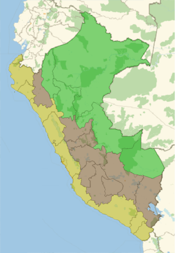
Traditional macro regions in Peru, that used to be taught in the 80’s, split Peru basically in 3 regions: costa (coast), sierra (mountain), selva (jungle). Even when this division is outdated (because not all the mountain is the same, or not all the jungle shares the same features), we can still group departments using that division to do some stats. This is how it is split:
In[]:=
GeoListPlot[classTradicional,PlotStyle(classTradicional/.plotStyleByClass),PlotLegendsSwatchLegend[classTradicional]]
Out[]=


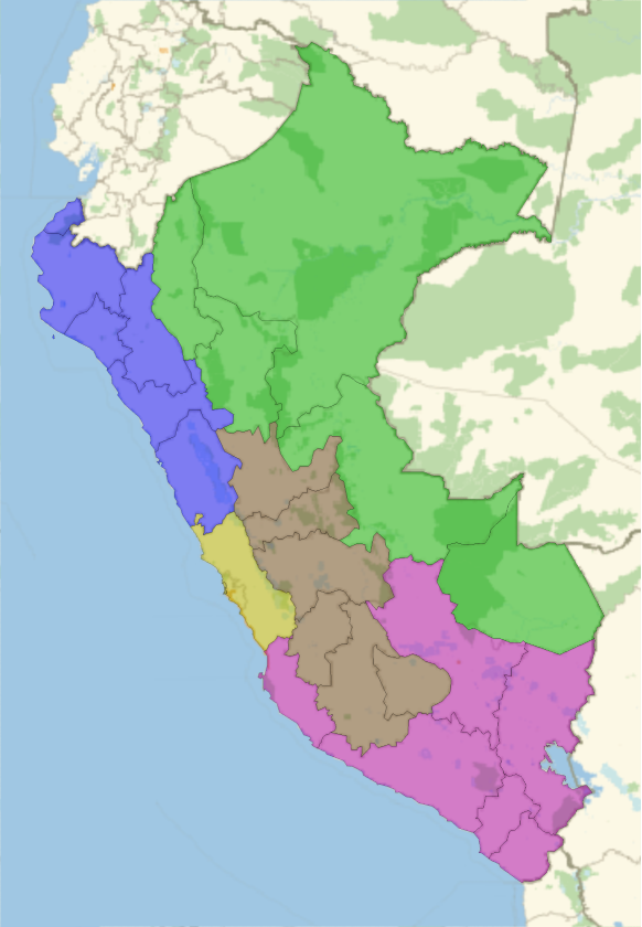
A bit more modern division is to split Peru in different macro regions:
In[]:=
GeoListPlot[classMacro,PlotStyle(classMacro/.plotStyleByClass),PlotLegendsSwatchLegend[classMacro]]
Out[]=


Plot code
Plot code
Plot COVID-19 progress by traditional divisions
Plot COVID-19 progress by traditional divisions
Confirmed cases
Confirmed cases
In[]:=
referenceNiceListLogPlotdataClasses[[Key/@classTradicionalPeru,"ConfirmadosT"]],"StartValue"10,
Out[]=


Deaths
Deaths
In[]:=
referenceNiceListLogPlotdataClasses[[Key/@classTradicionalPeru,"Fallecidos"]],"StartValue"3,
Out[]=
Average deaths per million
Average deaths per million
To avoid the noise of deaths per day, let’s take an average over a week:
Discussion
Discussion
Population is not evenly distributed among the regions:
And population density is totally different too:
Let’s take a look of the average elevation of the capital of each macro region:
In the coast and jungle there are a couple of outliers:
Now we can try a weighted average by population:
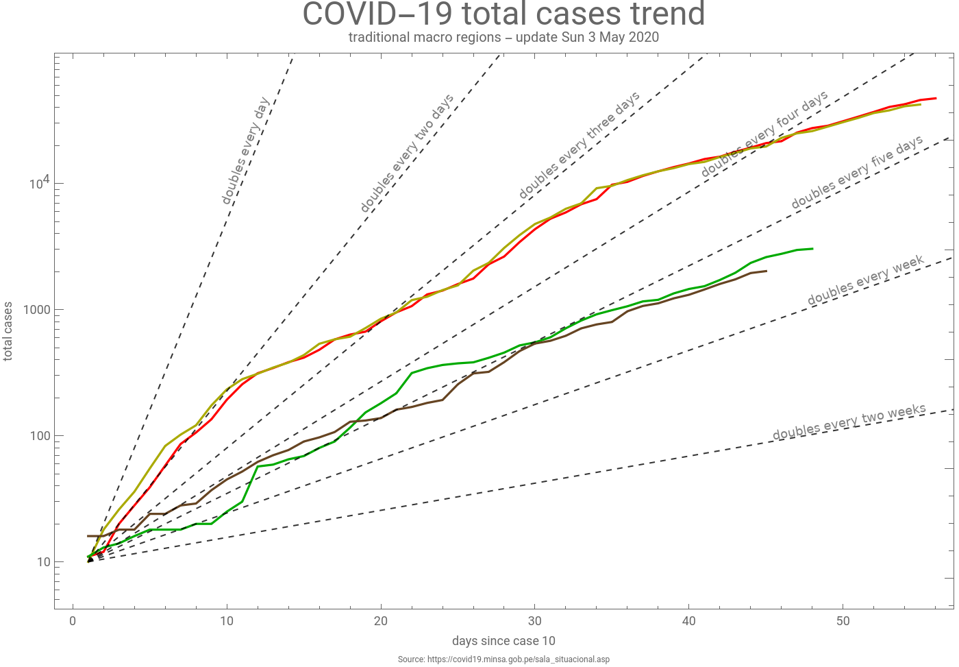
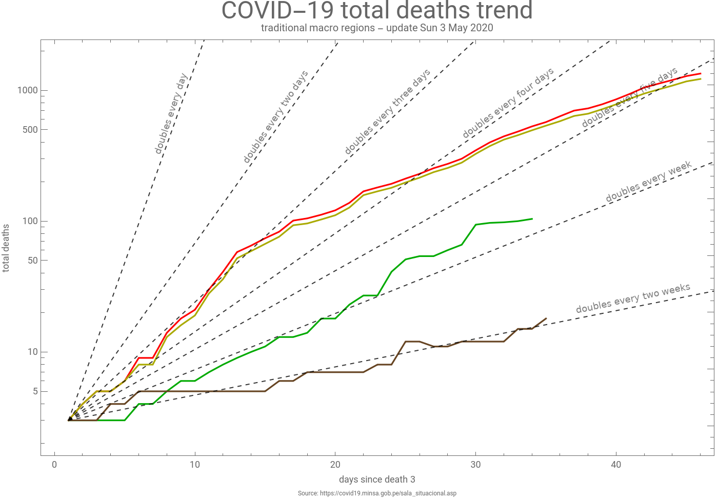
So, high population and high population density may explain why spread in the coast is higher than in the mountain or jungle, but spread trend in the jungle and mountain is quite similar, but deaths trend is totally different. There is already an article about how the elevation may play a role: https://www.sciencedirect.com/science/article/pii/S1569904820301014. These results may confirm a role, but I’m not sure yet if we can say that the influence is more because people is adapted to less oxygen or because weather helps stopping the propagation. We may need to split the data by province or district to properly classify each smaller region by elevation if we want to have more reliable results.
More data, plots and maps about COVID-19 in Peru can be found here: https://perucovid19.netlify.app.