Using experimental impulse response data, one can compute moments and normalized moments. This information can be used for process identification. We consider first order models, first order plus time delay models and second order models. Once the process parameters are found, we use NDSolve to obtain the solution to an impulse and compare it to the experimental data.
Acknowledgement: Experimental data were obtained from Process Dynamics, Modeling and Control, Ogunnaike and Ray, Oxford University Press, 1994.
Identification of a First Order Model using Moments
Identification of a First Order Model using Moments
Interpolation of experimental data
In[]:=
time={0.5,1,1.5,2,2.5,3,3.5,4,4.5,5,5.5,6,6.5,7};
In[]:=
ImpulseResponse={3.03,1.84,1.12,0.68,0.41,0.25,0.15,0.09,0.06,0.03,0.02,0.01,0.008,0.005};
In[]:=
tt=Transpose[{time,ImpulseResponse}]
Out[]=
{{0.5,3.03},{1,1.84},{1.5,1.12},{2,0.68},{2.5,0.41},{3,0.25},{3.5,0.15},{4,0.09},{4.5,0.06},{5,0.03},{5.5,0.02},{6,0.01},{6.5,0.008},{7,0.005}}
In[]:=
IR=Interpolation[tt,InterpolationOrder->1]
Out[]=
InterpolatingFunction


In[]:=
plt1=ListPlot[tt,PlotRange->All,PlotStyle->PointSize[0.02],Frame -> True,FrameLabel->{Style["time",16],Style["response",16]},GridLines->Automatic,AspectRatio->1,ImageSize->400{1,1}]
Out[]=
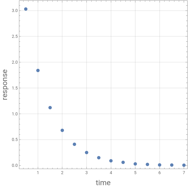
Computing time constant (τ) and gain (K)
We use some of the symbolic capabilities offered by Mathematica.
We use some of the symbolic capabilities offered by Mathematica.
In[]:=
f=InverseLaplaceTransform[K/(τs+1),s,t]
Out[]=
-
t
τ
τ
In[]:=
M0=Integrate[f,{t,0,Infinity}]
Out[]=
ConditionalExpression[K,Re[τ]>0]
In[]:=
μ
2
Out[]=
ConditionalExpression[2,Re[τ]>0]
2
τ
Computing moments and normalized moments
In[]:=
M
0
Out[]=
4.90525
In[]:=
M
1
Out[]=
5.03288
In[]:=
M
2
Out[]=
9.86047
In[]:=
μ
1
M
1
M
0
Out[]=
1.02602
In[]:=
μ
2
M
2
M
0
Out[]=
2.01019
In[]:=
τ=/2
μ
2
Out[]=
1.00254
In[]:=
K=
M
0
Out[]=
4.90525
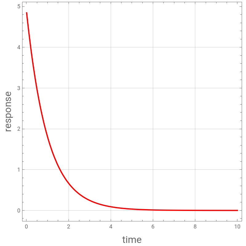
Obtaining the impulse response of the first order system with τ=1.002 and K=4.905
In[]:=
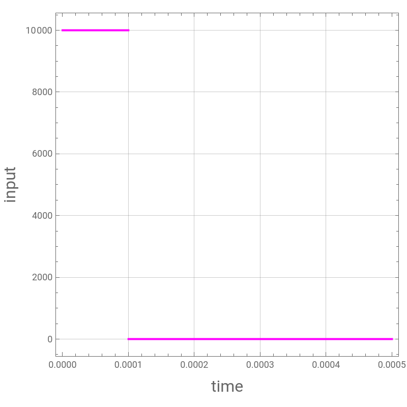
u[t_]:=ϵ (UnitStep[t]-UnitStep[t-1/ϵ])
In[]:=
ϵ=10000;
In[]:=
Plot[u[t],{t,0,5/ϵ},PlotStyle->{Thick,RGBColor[1,0,1]},Frame -> True,FrameLabel->{Style["time",16],Style["input",16]},GridLines->Automatic,AspectRatio->1,ImageSize->400{1,1}]
Out[]=
In[]:=
Clear[f]
In[]:=
sol=NDSolve[{τ f'[t]+f[t]K u[t],f[0]0},f[t],{t,0,10}]
Out[]=
f[t]InterpolatingFunction[t]

In[]:=
plt2=Plot[f[t]/.sol,{t,0.01,10},PlotRange->All,PlotStyle->{Thick,RGBColor[1,0,0]},FrameLabel->{Style["time",16],Style["response",16]},
Frame -> True,GridLines->Automatic,AspectRatio->1,ImageSize->400{1,1}]
Frame -> True,GridLines->Automatic,AspectRatio->1,ImageSize->400{1,1}]
Out[]=
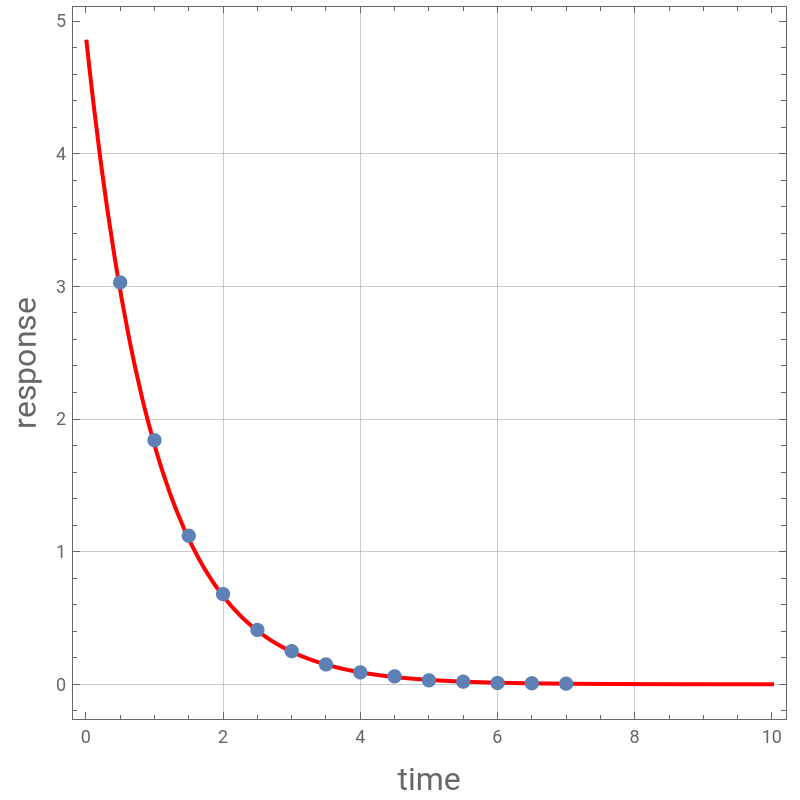
Comparing experimental data and data obtained from process identification
In[]:=
Show[plt2,plt1]
Out[]=
Identification of a First Order Model with Time Delay using Moments
Identification of a First Order Model with Time Delay using Moments
Acknowledgement: Experimental data were obtained from Process Dynamics, Modeling and Control, Ogunnaike and Ray, Oxford University Press, 1994.
Interpolation of experimental data
In[]:=
time={0,0.5,1,1.5,2,2.5,3,3.5,4,4.5,5,5.5,6,6.5,7,7.5,8,8.5,9,9.5,10};
In[]:=
ImpulseResponse={0,0,0,0,10.10,6.36,3.86,2.36,1.43,0.86,0.53,0.31,0.19,0.13,0.06,0.042,0.021,0.017,0.011,0.006,0.003};
In[]:=
tt=Transpose[{time,ImpulseResponse}];
In[]:=
IR=Interpolation[tt,InterpolationOrder->1]
In[]:=
plt1=ListPlot[tt,PlotRange->All,PlotStyle->PointSize[0.02],FrameLabel->{Style["time",16],Style["response",16]},
Frame -> True,GridLines->Automatic,AspectRatio->1,ImageSize->400{1,1}]
Frame -> True,GridLines->Automatic,AspectRatio->1,ImageSize->400{1,1}]
Computing moments and normalized moments
Computing time constant (τ) gain (K) and delay (α)
We use some of the symbolic capabilities offered by Mathematica.
We use some of the symbolic capabilities offered by Mathematica.
Obtaining the impulse response of the first order system with τ=1.002, α=1.778 and K=13.144
In[]:=
u[t_]:=ϵ (UnitStep[t]-UnitStep[t-1/ϵ])
In[]:=
Plot[u[t],{t,0,5/ϵ},PlotStyle->{Thick,RGBColor[1,0,1]},FrameLabel->{Style["time",16],Style["input",16]},Frame -> True,GridLines->Automatic,AspectRatio->1,ImageSize->400{1,1}]
In[]:=
sol2=NDSolve[{τ f'[t]+f[t]K u[t-α],f[α]0},f[t],{t,α,10}]
In[]:=
plt2=Plot[f[t]/.sol2,{t,α,10},PlotStyle->{Thick,RGBColor[1,0,0]},PlotRange->All,PlotStyle->PointSize[0.02],
Frame->True,FrameLabel->{Style["time",16],Style["response",16]},GridLines->Automatic,AspectRatio->1,ImageSize->400{1,1}]
Frame->True,FrameLabel->{Style["time",16],Style["response",16]},GridLines->Automatic,AspectRatio->1,ImageSize->400{1,1}]
In[]:=
Show[plt2,plt1]
Second Order Model Identification using Moments
Second Order Model Identification using Moments
Interpolation of experimental data
In[]:=
time={0,0.5,1,1.5,2,2.5,3,3.5,4,4.5,5,5.5,6,6.5,7,7.5,8,8.5,9,9.5,10,10.5,11,11.5,12,12.5,13,13.5,14,14.5,15,15.5,16,16.5,17,17.5,18,18.5,19,19.5,20};
In[]:=
ImpulseResponse={0,0.1215,0.1982,0.2392,0.2530,0.2470,
0.2278,0.2006,0.1694,0.1375,0.1070,0.0793,0.0553,0.0353,0.0193,0.0070,-0.0018,-0.0079,-0.0116,-0.0135,-0.0139,
-0.0134,-0.0122,-0.0106,-0.0089,-0.0071,-0.0055,-0.0040,-0.0027,-0.0017,-0.0008,-0.0002,0.0001,0.0004,0.0006,
0.0007,0.0007,0.0007,0.0006,0.0005,0.0004};
0.2278,0.2006,0.1694,0.1375,0.1070,0.0793,0.0553,0.0353,0.0193,0.0070,-0.0018,-0.0079,-0.0116,-0.0135,-0.0139,
-0.0134,-0.0122,-0.0106,-0.0089,-0.0071,-0.0055,-0.0040,-0.0027,-0.0017,-0.0008,-0.0002,0.0001,0.0004,0.0006,
0.0007,0.0007,0.0007,0.0006,0.0005,0.0004};
In[]:=
tt=Transpose[{time,ImpulseResponse}];
In[]:=
IR=Interpolation[tt,InterpolationOrder->1]
In[]:=
plt1=ListPlot[tt,PlotRange->All,PlotStyle->PointSize[0.02],Frame->True,FrameLabel->{Style["time",16],Style["response",16]},GridLines->Automatic,AspectRatio->1,ImageSize->400{1,1}]
Computing moments and normalized moments
Computing second order model parameters
We use some of the symbolic capabilities offered by Mathematica.
We use some of the symbolic capabilities offered by Mathematica.
In[]:=
u[t_]:=ϵ (UnitStep[t]-UnitStep[t-1/ϵ])
In[]:=
Plot[u[t],{t,0,5/ϵ},PlotStyle->{Thick,RGBColor[1,0,1]},Frame->True,FrameLabel->{Style["time",16],Style["input",16]},GridLines->Automatic,AspectRatio->1,ImageSize->400{1,1}]
In[]:=
plt2=Plot[f[t]/.sol2,{t,0,20},PlotStyle->{Thick,RGBColor[1,0,0]},
Frame->True,FrameLabel->{Style["time",16],Style["response",16]},GridLines->Automatic,AspectRatio->1,ImageSize->400{1,1}]
Frame->True,FrameLabel->{Style["time",16],Style["response",16]},GridLines->Automatic,AspectRatio->1,ImageSize->400{1,1}]
In[]:=
Show[plt1,plt2]
CITE THIS NOTEBOOK
CITE THIS NOTEBOOK
Process identification using impulse response and normalized moments
by Housam Binous and Ahmed Bellagi
Wolfram Community, STAFF PICKS, February 18, 2024
https://community.wolfram.com/groups/-/m/t/3125234
by Housam Binous and Ahmed Bellagi
Wolfram Community, STAFF PICKS, February 18, 2024
https://community.wolfram.com/groups/-/m/t/3125234