The Central Limit Theorem

Stephen Wolfram
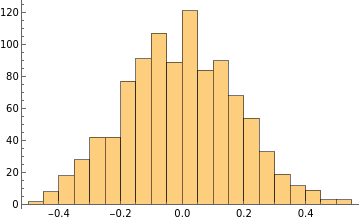
The Central Limit Theorem is an important result in statistics that states that subject to certain conditions, averages of multiple random variables tend to follow a normal distribution.

Discovering the Central Limit Theorem

Let’s “discover” the Central Limit Theorem empirically, by looking at collections of random numbers.
Make a list of 10 random real numbers between -1 and 1:
In[]:=
RandomReal[{-1,1},10]
Out[]=
{-0.0771015,-0.366985,-0.339309,0.828772,-0.0314546,0.258496,-0.626615,0.903993,0.337799,-0.719367}
These random numbers are uniformly distributed, so if we make a histogram of them, it’ll be flat.
Make a histogram of 1000 random numbers between -1 and 1:
In[]:=
Histogram[RandomReal[{-1,1},1000]]
Out[]=
With 100,000 numbers the histogram is almost exactly flat:
In[]:=
Histogram[RandomReal[{-1,1},100000]]
Out[]=
Now let’s start finding means of collections of numbers.
This finds the mean of 10 random real numbers:
In[]:=
Mean[RandomReal[{-1,1},10]]
Out[]=
-0.112097
Here is a list of 10 such means:
In[]:=
Table[Mean[RandomReal[{-1,1},10]],10]
Out[]=
{-0.112467,0.0172069,0.0826008,0.134617,-0.220979,-0.0600067,-0.14143,0.171051,-0.13263,0.0301039}
Here is the distribution of 1000 such means:
In[]:=
Histogram[Table[Mean[RandomReal[{-1,1},10]],1000]]
Out[]=
Here is the distribution for 100,000 means:
In[]:=
Histogram[Table[Mean[RandomReal[{-1,1},10]],100000]]
Out[]=
The distribution for the means is not flat; instead it’s a bell-shaped curve.
It’s easier to see the shape of the curve if we use smaller bins; here width 0.01:
In[]:=
Histogram[Table[Mean[RandomReal[{-1,1},10]],100000],{.01}]
Out[]=
If we only put 5 numbers into the mean, we still get a very similar result:
In[]:=
Histogram[Table[Mean[RandomReal[{-1,1},5]],100000],{.01}]
Out[]=
The crucial thing about the Central Limit Theorem is that it holds for a wide range of different underlying random distributions.
If we cube each random number, the distribution of the results isn’t flat:
In[]:=
Histogram[Table[RandomReal[{-1,1}]^3,1000]]
Out[]=
The distribution of the means is still the same shape:
In[]:=
Histogram[Table[Mean[Table[RandomReal[{-1,1}]^3,10]],100000],{.01}]
Out[]=
If we square each number, we’ll always get results that are positive:
The distribution of the means is still the same shape, though its center (mean) is shifted: