Undergraduate Physics Education | Things to Try
Undergraduate Physics Education | Things to Try
Make edits and run any piece of code by clicking inside the code and pressing .
+
Solve a Mass-Spring System
Solve a Mass-Spring System
The governing equation of motion is derived from Newton's second law x=-x(t), where is the angular frequency.
2
d
d
2
t
2
ω
ω=
k/m
Solve the equation, subject to initial conditions:
In[]:=
eqn=x''[t]==-x[t];sol=DSolveValue[{eqn,x[0]==x0,x'[0]==v0},x[t],t]
2
ω
Out[]=
x0ωCos[tω]+v0Sin[tω]
ω
Rewrite the solution in terms of amplitude and phase angle ϕ:
A
In[]:=
x[t_]=Simplify[sol/.{x0->ACos[ϕ],v0->-ωASin[ϕ]}];x[t]
Out[]=
ACos[ϕ+tω]
Get the velocity and acceleration as the first and second derivatives of position with respect to time:
In[]:=
v[t_]=D[x[t],{t,1}];v[t]
Out[]=
-AωSin[ϕ+tω]
In[]:=
a[t_]=D[x[t],{t,2}];a[t]
Out[]=
-ACos[ϕ+tω]
2
ω
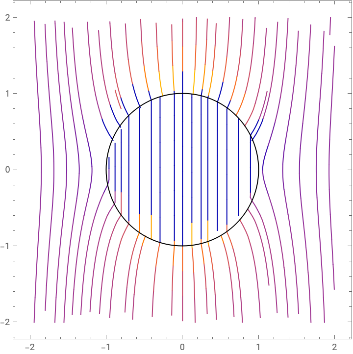
Plot the electric field lines of a dielectric ball in an electric field
Plot the electric field lines of a dielectric ball in an electric field
The formula for the electric field near a dielectric ball can be obtained through :
In[]:=
field=
Out[]=
|
Substitute in values for all expressions in the result above:
In[]:=
elecField[x_,y_,z_]:=field/.QuantityVariable["R","Radius"]->1,QuantityVariable[Subscript["E",0],"ElectricFieldStrength"]->2,->4,QuantityVariable["x","Length"]->x,QuantityVariable["y","Length"]->y,QuantityVariable["z","Length"]->z
ϵ
Use to visualize the electric field lines for this physical scenario:
In[]:=
StreamPlot[elecField[x,0,z][[{1,3}]]//N,{x,-2,2},{z,-2,2},StreamMarkers->None,Epilog->Circle[],StreamColorFunctionScaling->True]
Out[]=
Solve the Schrödinger Equation for the Linear Harmonic Oscillator
Solve the Schrödinger Equation for the Linear Harmonic Oscillator
The Schrödinger equation for the linear harmonic oscillator is given by:+ψ(x)=ϵψ(x)
-ψ"(x)
2
ℏ
2m
k
2
2
x
For simplicity scale the variables such that :
ℏ=m=k=1
In[]:=
ℒ=-ψ''[x]+ψ[x];
1
2
1
2
2
x
Use the algorithm to get the first five eigenvalues and eigenfunctions:
In[]:=
{evals,efns}=NDEigensystem[ℒ,ψ[x],{x,-5,5},5];
List the eigenvalues (the exact values are known to be , …):
ϵ=,,
1
2
3
2
5
2
In[]:=
evals
Out[]=
{0.500079,1.50054,2.5019,3.5047,4.50941}
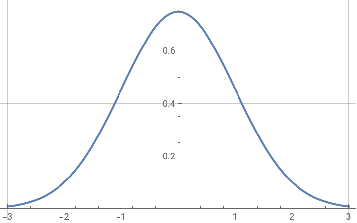
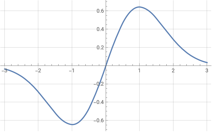
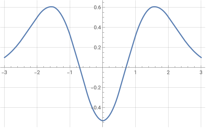
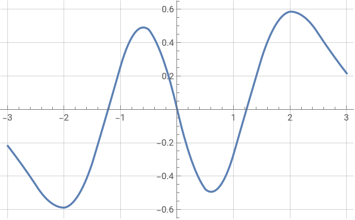
Plot the first four eigenfunctions:
In[]:=
Table[Plot[Evaluate[-efns[[n]]],{x,-3,3},GridLines->Automatic],{n,1,4}]
Out[]=
,
,
,
Interactive demonstrations
Interactive demonstrations
Find demonstrations based on keywords:
In[]:=
EntityList[FilteredEntityClass["WolframDemonstration",EntityFunction[c,MemberQ[c["Keywords"],"force"]]]]
Out[]=
,,,,,,,,,,,,,,,,,,,,,,,,,,,,,,,,,,,,,

Get a list of all demonstration classes and display a random sample of 10:
In[]:=
ecl=EntityClassList["WolframDemonstration"];RandomSample[ecl,10]
Out[]=
,,,,,,,,,

List all demonstrations in the class of interest:
In[]:=
el=EntityList;RandomSample[el,10]
Out[]=
,,,,,,,,,

Interact with a particular demonstration: