Wolfram for Environmental Science | Things to Try
Wolfram for Environmental Science | Things to Try
Make edits and run any piece of code by clicking inside the code and pressing .
+
Access & Analyze Weather and Climate Data
Access & Analyze Weather and Climate Data
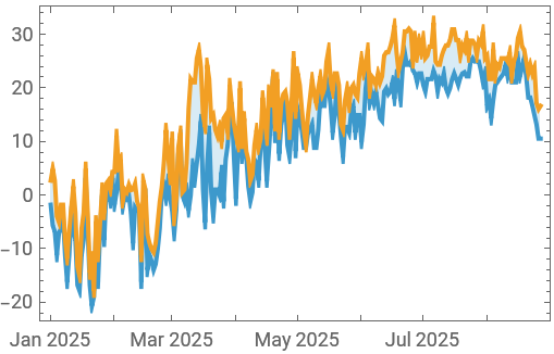
Retrieve temperature data for a provided location over a specified temporal range: |
In[]:=
min=WeatherData,"MinTemperature",,,"Day";max=WeatherData,"MaxTemperature",,,"Day";
Make a time series plot of the data: |
In[]:=
DateListPlot[{min,max},Joined->True,Filling->{1->{2}},PlotLegends->SwatchLegend[{,},{"Min °C","Max °C"}]]

Out[]=


Import atmospheric CO 2 |
In[]:=
noaaCO2Data=CastColumns[Import["https://gml.noaa.gov/webdata/ccgg/trends/co2/co2_mm_mlo.csv","Tabular"],{"year"->"Integer16","Month"->"Integer8"}]
Out[]=
Tabular


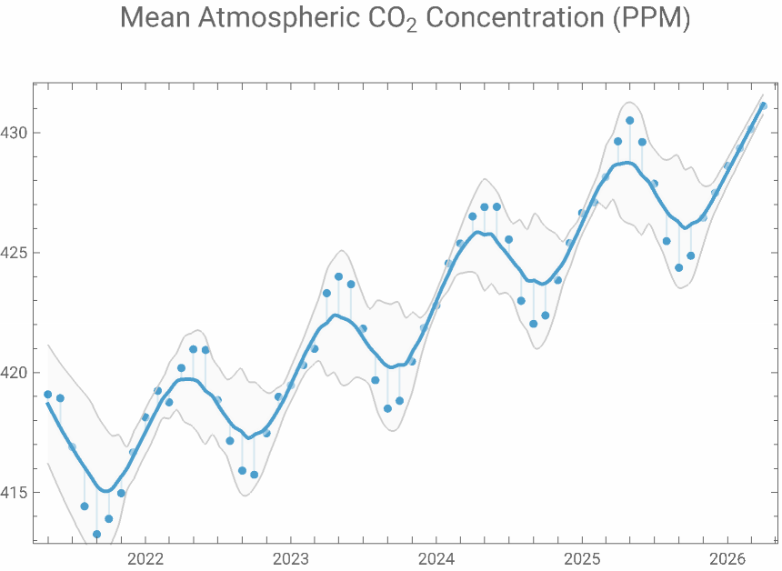
Plot a time series of atmospheric CO 2 |
In[]:=
featurekeelingCurve=DateListPlotTake[Normal[Dataset[TransformColumns[noaaCO2Data,"date"->Function[DateObject[{#year,#month},"Month"]]][All,{"date","average"}]][All,{#date,#average}&]],-60],
Out[]=
Make Maps and Access Remote Sensing Services
Make Maps and Access Remote Sensing Services
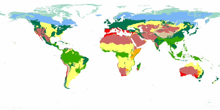
Map global ecological regions such as terrestrial biomes: |
In[]:=
biomes=->,->,->,->,->,->,->,->,->;GeoGraphics[{GeoStyling[#〚2〛],EntityValue[#〚1〛,"Polygon"]}&/@biomes,GeoBackground->Transparent,ImageSize->450]
Out[]=
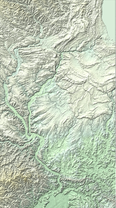
Plot a relief map of Illinois: |
In[]:=
GeoGraphics,GeoBackground->"ReliefMap",GeoZoomLevel->8
Out[]=
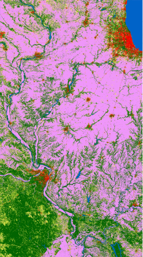
Map land cover using ESA data: |
In[]:=
LegendedGeoGraphics,GeoServer->,GeoZoomLevel->8,SwatchLegend[{,,,,,,,,,,},{"Tree cover","Shrubland","Grassland","Cropland","Built-up","Bare / sparse vegetation","Snow and ice","Permanent water bodies","Herbaceous wetland","Mangroves","Moss and lichen"},LegendLayout->{"Column",1}]
Out[]=


Model Environmental and Ecological Processes
Model Environmental and Ecological Processes