Engineering Education | Things to Try
Engineering Education | Things to Try
Make edits and run any piece of code by clicking inside the code and pressing .
+
Solve a differential equation
Solve a differential equation
Model the motion of a pendulum in Cartesian coordinates. Derive the governing equations using Newton’s second law of motion, m ′ ′ x F x m ′ ′ y F y |
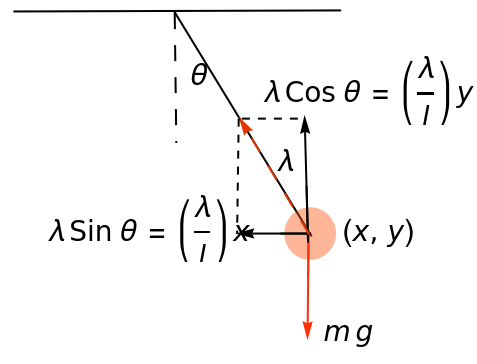
Define the equation, set up the algebraic constraint and initial conditions: |
In[]:=
deqns={x''[t]λ[t]x[t],y''[t]λ[t]y[t]-9.81};aeqns={+};ics={x[0]1,y'[0]1};
2
x[t]
2
y[t]
2
1
Use |
In[]:=
sol1=NDSolve[{deqns,aeqns,ics},{x,y,λ},{t,0,5},Method{"IndexReduction"True}]
Out[]=
xInterpolatingFunction,yInterpolatingFunction,λInterpolatingFunction


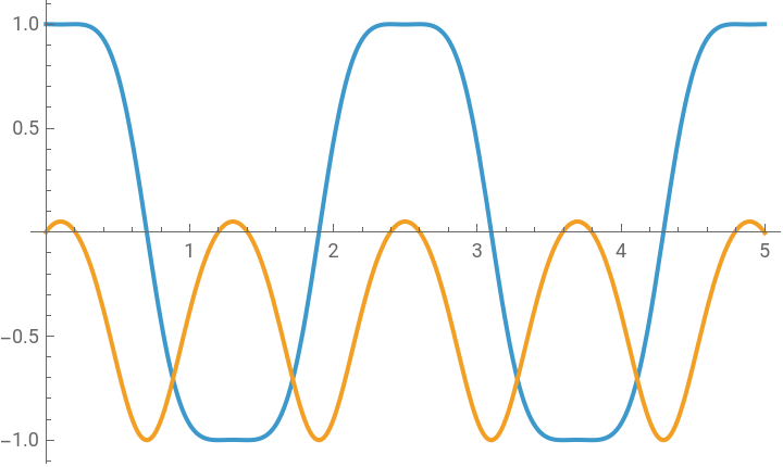
Visualize the displacement in both x and y direction about time: |
In[]:=
Plot[Evaluate[{x[t],y[t]}/.sol1],{t,0,5}]
Out[]=
Interactive demonstrations for mechanical engineering
Interactive demonstrations for mechanical engineering
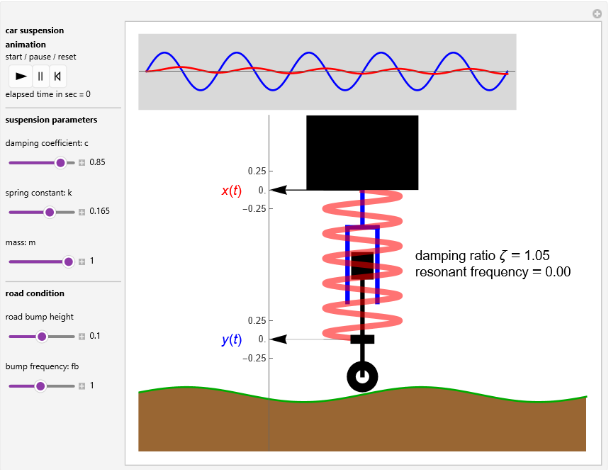
Simulating vehicle suspension with a simplified quarter-car model: |
In[]:=
ResourceData["Demonstration: Simulating Vehicle Suspension with a Simplified Quarter-Car Model"]
Out[]=
Interactive demonstrations for electrical engineering
Interactive demonstrations for electrical engineering
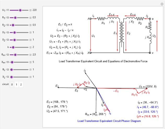
A power source supplies a voltage that is some combination of sine waves, represented by a phasor diagram. For sin(x), the phasor diagram would be a unit vector rotating about the origin. A more complex circuit gives a combination of these, representing the changes in electromagnetic quantities as circuit parameters are varied. |
In[]:=
ResourceData["Demonstration: Circuit Phasor Diagram for Transformers"]
Out[]=
Signal processing
Signal processing
FIR filters applied to an audio object:
In[]:=
a=ExampleData[{"Audio","Apollo11ReturnSafely"},"Audio"];lp=LowpassFilter[a,,101];hp=HighpassFilter[a,,101];bs=BandstopFilter[a,,,91];
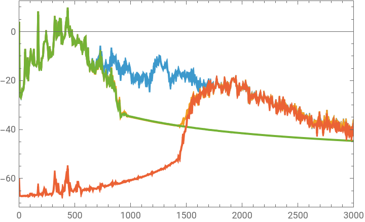
Plot the periodogram of the original and processed signals:
In[]:=
Periodogram[{a,bs,lp,hp},2000,PlotRange{{0,3000},Automatic},FrameTrue,ImageSizeMedium,PlotLegends{"Original","Bandstop","Lowpass","Highpass"}]
Out[]=


System design and control theory
System design and control theory
Define the equations of motion for a pendulum on a wheel (like a Segway): |
In[]:=
diffeqs={-lmSin[θ[t]][t]-(m+M)[t]+lmCos[θ[t]][t]F[t],-gSin[θ[t]]-Cos[θ[t]][t]+l[t]0}
2
′
θ
′′
x
′′
θ
′′
x
′′
θ
Out[]=
{-lmSin[θ[t]][t]-(m+M)[t]+lmCos[θ[t]][t]F[t],-gSin[θ[t]]-Cos[θ[t]][t]+l[t]0}
2
′
θ
′′
x
′′
θ
′′
x
′′
θ
Create a dynamic model by specifying states, inputs, outputs and parameter values: |
In[]:=
system=NonlinearStateSpaceModel[diffeqs,{θ[t],x[t]},F[t],{θ[t],x[t]},t]/.{M->10,m->80,l->1,g->9.8}
Out[]=

θ[t] | x. 1 |
x. 1 | - 882.Sin[θ[t]] -90+80 2 Cos[θ[t]] Cos[θ[t]]F[t]+80Sin[θ[t]] 2 x. 1 -90+80 2 Cos[θ[t]] |
x[t] | x. 2 |
x. 2 | - 784.Cos[θ[t]]Sin[θ[t]] -90+80 2 Cos[θ[t]] F[t]+80Sin[θ[t]] 2 x. 1 -90+80 2 Cos[θ[t]] |
θ[t] | |
x[t] |
Choose poles in the left-half plane for the closed-loop system: |
In[]:=
p={-1+2I,-1-2I,-0.35+0.35I,-0.35-0.35I}