Wolfram for Civil Engineering | Things to Try
Wolfram for Civil Engineering | Things to Try
Make edits and run any piece of code by clicking inside the code and pressing .
+
Civil Engineering Computation & Modeling. For everyone from students learning the fundamentals to practicing engineers and research teams. A single workflow for structural mechanics, hydraulics, and infrastructure systems—combining symbolic derivations, high-performance numerical simulation, and rigorous units-aware calculations with interactive visualization and real-world data, so you can go from assumptions to validated designs and decisions faster.
Find the properties of materials
Find the properties of materials
Wolfram provides detailed information about more than 11,000 kinds of alloys, in response to simple, natural-language queries.
Find the thermodynamic property of water at standard pressure: |
In[]:=
ThermodynamicData["Water","ThermalConductivity",{"Temperature"->Quantity[375,"Kelvins"]}]
Find the Young’s modulus of steel: |
In[]:=
WolframAlpha["Young's modulus of steel"]
Find the Young’s modulus of titanium: |
In[]:=
WolframAlpha["Young's modulus of titanium"]
Find the thermodynamic property of water at standard pressure: |
In[]:=
WolframAlpha["UNS G10500 tensile yield strength"]
Use Built-in Physics Formulas
Use Built-in Physics Formulas
Compute the moment of inertia of the unit disk centered at the origin about the x-axis: |
In[]:=
Compute the miles per gallon equivalent for a typical electric vehicle driving on highway: |
In[]:=
ColumnFormulaData["MPGe","QuantityVariableNames"],FormulaData["MPGe"],FormulaData"MPGe","D"->,"E"->
Out[]=
{ MPGe D V E |
MPGe D V V E |
MPGe V |
Convert Between Units (use a single UnitConvert merged with above)
Convert Between Units (use a single UnitConvert merged with above)
Convert the Young’s modulus of steel from emprical unit in to metric system: |
In[]:=
UnitConvert,"Gigapascals"
Convert the power of common gas oven from BTU to Joules: |
In[]:=
UnitConvert[Quantity[20000.,"BritishThermalUnits59F"],"Joules"]
Out[]=
Convert between compound units for milage efficiency: |
In[]:=
UnitConvert[Quantity[30.,"Miles"/"Gallons"],"Kilometers"/"Liters"]
Out[]=
Solve Differential Equations for Beam Deflection
Solve Differential Equations for Beam Deflection
Symbolically solve for beding and shearing stresses in an Euler Bernoulli cantilever beam with Young’s modulus E=20Gpa |
In[]:=
M=EI*D[y[x],{x,2}];V=EI*D[y[x],{x,3}];th=EI*D[y[x],x];sol=DSolveValue[{EI*y''''[x]==0,y[0]==0,y'[0]==0,EI*y'''[L]==125,y''[L]==0},y[x],x]
Out[]=
-
125(3L-)
2
x
3
x
6EI
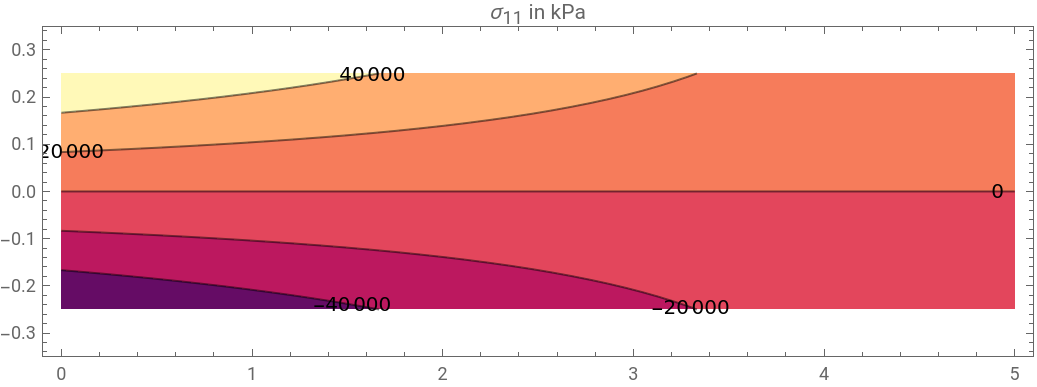
If the length of the beam is 5 meter, the height of the beam is 0.5 m, while the width is 0.25, plot the Cauchystresstensorcomponent σ 11 |
In[]:=
moi=[0.25,0.5];ei=20*10^6*moi;sol=Expand[sol/.{L->5,EI->ei}];s11=-20*10^6*D[sol,{x,2}]*x2;ContourPlots11,{x,0,5},{x2,-0.25,0.25},
Out[]=
In[]:=
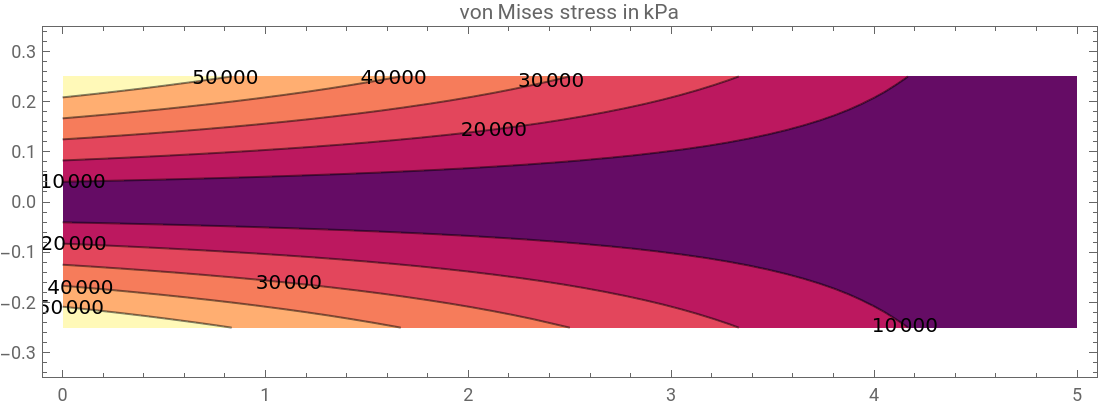
vq=(0.5/2-x2)*0.25*(x2/2+0.5/4);s12=-20*10^6*D[sol,{x,3}]*vq/0.25;sm={{s11,s12},{s12,0}};ContourPlotVonMisesStress{{u[x,y,z],v[x,y,z],w[x,y,z]},{x,y,z}},<|"YoungModulus"Y.,"PoissonRatio"ν.|>,sm,{x,0,5},{x2,-0.25,0.25},
Out[]=
Find Principle Stress using Eigensystem
Find Principle Stress using Eigensystem
Find the principle stresses using eigensystem for the cantilever beam above at given locations: |
In[]:=
Column[MatrixForm/@(With[{s11=240000.*x2-48000.x1*x2,s12=-1500.+24000.x2^2},Eigensystem[{{s11,s12,0},{s12,0,0},{0,0,0}}/.{x1->#1,x2->#2}]]&@@@{{0,0.25},{0,-0.25/2},{0,.25/2}})]
Out[]=
| ||||||
| ||||||
|