Wolfram for Chemical Engineering | Things to Try
Wolfram for Chemical Engineering | Things to Try
Make edits and run any piece of code by clicking inside the code and pressing + .
Chemical Engineering Computation & Modeling. For everyone from students learning the fundamentals to practising engineers and research teams. A single workflow for thermophysical properties, material and energy balances, phase equilibrium, reaction engineering, transport phenomena and process dynamics—combining symbolic derivations, numerical simulation, units-aware calculations, interactive visualization and experimental data analysis.
Find properties of chemicals and fluids
Find properties of chemicals and fluids
Find the molecular formula, molar mass, normal boiling point and density of methanol:
In[]:=
ChemicalData["Methanol",#]&/@{"CompoundFormulaString","MolarMass","BoilingPoint","Density"}
Out[]=
CH4O,,,
Typing “=[...]” lets you look up a compound from its common synonym using natural language:
In[]:=
=[thf]
Out[]=
Find the dynamic viscosity of air at 300 K and 0.2 MPa:
In[]:=
ThermodynamicData["Air","DynamicViscosity",{"Pressure"->Quantity[0.2,"Megapascals"],"Temperature"->Quantity[300,"Kelvins"]}]
Out[]=
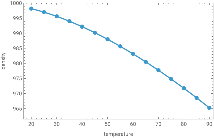
Plot the density of liquid water between 20°C and 90°C:
In[]:=
temperatures=Quantity[Range[20,90,5],"DegreesCelsius"];
In[]:=
densities=ThermodynamicData["Water","MassDensity",{"Temperature"->temperatures}];
In[]:=
ListLinePlot[Transpose[{temperatures,densities}],Frame->True,FrameLabel->{"temperature","density"},PlotMarkers->Automatic]
Out[]=
Calculate with units, formulas and dimensionless groups
Calculate with units, formulas and dimensionless groups
Convert between different units:
In[]:=
UnitConvert[Quantity[3.5,"Megawatts"],"InternationalTableBritishThermalUnits"/"Hours"]
Out[]=
In[]:=
UnitConvert[Quantity[1.2,"Centipoise"],"Pascals""Seconds"]
Out[]=
In[]:=
UnitConvert[Quantity[250,"Kilomoles"/"Hours"],"Moles"/"Seconds"]
Out[]=
Retrieve the Reynolds-number equation and identify its variables and their dimensions:
In[]:=
With[{f={"ReynoldsNumber","DynamicViscosity"}},Column[{FormulaData[f],FormulaData[f,"QuantityVariableNames"],FormulaData[f,"QuantityVariableDimensions"]}]]
Out[]=
Re l v ρ η |
{ Re l v η ρ |
{ Re l v η ρ |
Calculate the Reynolds number for water flowing at 2 m/s through a 50 mm pipe:
In[]:=
density=Quantity[998,"Kilograms"/"Meters"^3];
In[]:=
velocity=Quantity[2,"Meters"/"Seconds"];
In[]:=
diameter=Quantity[50,"Millimeters"];
In[]:=
viscosity=Quantity[1,"Centipoise"];
In[]:=
reynoldsNumber=densityvelocitydiameter/viscosity
Out[]=
99800
Calculate the required heat-transfer area for a specified duty, overall coefficient and terminal temperature differences using the log-mean temperature difference (LMTD) method:
In[]:=
duty=Quantity[2.5,"Megawatts"];
In[]:=
overallCoefficient=Quantity[500,"Watts"/("Meters"^2"Kelvins")];
In[]:=
deltaT1=Quantity[70,"Kelvins"];
In[]:=
deltaT2=Quantity[30,"Kelvins"];
In[]:=
logMeanTemperatureDifference=(deltaT1-deltaT2)/Log[deltaT1/deltaT2];
In[]:=
area=UnitConvert[duty/(overallCoefficientlogMeanTemperatureDifference),"Meters"^2]
Out[]=
Solve a material balance and flash calculation
Solve a material balance and flash calculation
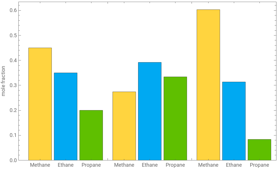
Here is a simple flash calculation to determine vapour and liquid fractions for a three-component feed.
Specify feed components and overall composition:
In[]:=
components={"Methane","Ethane","Propane"};
In[]:=
z={0.45,0.35,0.20};
Assume we know the vapour/liquid ratios for each component:
In[]:=
kValues={2.2,0.8,0.25};
Solve the Rachford-Rice equations for vapor fraction:
In[]:=
vaporFraction=vf/.FindRoot[Total[z(kValues-1)/(1+vf(kValues-1))]==0,{vf,0.5}];
Determine phase compositions:
In[]:=
x=z/(1+vaporFraction(kValues-1));
In[]:=
y=kValuesx;
Collect results:
In[]:=
Column[{Row[{"vapour fraction = ",vaporFraction}],Dataset@MapThread[<|"component"->#1,"feed z"->#2,"liquid x"->#3,"vapour y"->#4|>&,{components,z,x,y}]}]
Out[]=
vapour fraction = 0.534926 | ||||||||||||||||||
Visualize:
In[]:=
BarChart[{z,x,y},ChartLegends->{"feed","liquid","vapour"},ChartLabels->components,Frame->True,FrameLabel->{None,"mole fraction"}]
Out[]=


Solve differential equations for a reaction system
Solve differential equations for a reaction system
Define equations relating concentrations of species , , :
A
B
C
In[]:=
equations={ca'[t]==-k1ca[t],cb'[t]==k1ca[t]-k2cb[t],cc'[t]==k2cb[t]};
Specify initial conditions:
In[]:=
initConds={ca[0]==ca0,cb[0]==0,cc[0]==0};
Solve symbolically:
Make an interactive plot of the concentration profiles:
Find the natural modes of the reaction network:
Visualize heat or mass transfer
Visualize heat or mass transfer
In chemical engineering it is often necessary to model diffusion phenomena. Here we simulate the evolution of concentration in a one-dimensional slab starting from an initial distribution and with both ends maintaining zero concentration.
Clear variables from previous example:
Define the diffusivity in the slab:
Solve the one-dimensional diffusion equation for concentration profile:
Visualize the profile over time as a series of snapshots:
Visualize diffusion over time as a density plot:
Fit models to experimental data
Fit models to experimental data
Start with a reaction-rate data set:
Carry out a nonlinear fit:
Inspect the parameters:
Compare fit and data:
Analyze real-world data
Analyze real-world data
Here we demonstrate Wolfram Language’s powerful data science capabilities on a real-world dataset of industrial boiler time-series data.
Connect to the data source on Kaggle:
Inspect the files in the dataset:
Download the data and wrangle into a convenient form, with columns nicely labeled:
This dataset contains many columns corresponding to various sensors in the boiler:
We’ll initially consider several representative sensors:
Let’s visualize their behavior as a time series:
Characterize their distributions:
Now let’s investigate the correlation between the six upper furnace pressure sensors:
Finally, we can use anomaly detection to flag states which may signal an operational issue: