Wolfram 可视化 | 应用示例
Wolfram 可视化 | 应用示例
在代码中点击并按下 ,即可编辑并运行任何代码。
+
科学、数据与函数可视化。Wolfram 可视化功能简化并自动化图表创建过程,帮助用户理解数据和函数,适用于从个人探索到报告撰写和学术论文发表等各种场景。
可视化数据探索
可视化数据探索
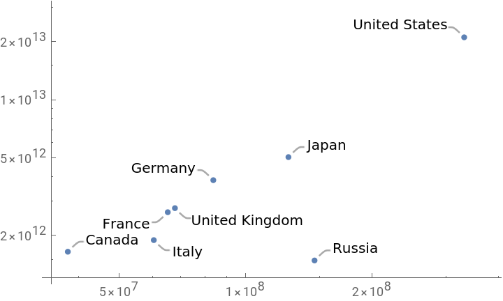
使用数十种可用图表类型可视化数据趋势: |
ListPlot[{"Population","GDP"}]["Name"],ScalingFunctions{"Log","Log"}

Out[]=
轻松使用饼图可视化比例关系: |
PieChart["Population"],ChartLabels->["Name"]
轻松使用柱状图比较不同类别的数据: |
BarChart["Population"],ChartLabels->["CountryCode"]
在多层组织结构中标记和可视化数据: |
BarChart,,ChartLabels->["CountryCode"],None,ChartLegends->{"2005","2020"}

设置绘图样式
设置绘图样式
定义并绘制一组函数: |
functions=Table[BesselJ[n,x],{n,4}];Plot[Evaluate[functions],{x,0,10}]
使用 |
Plot[Evaluate[functions],{x,0,10},PlotTheme->"Detailed"]
创建显示不同主题的列表以便于比较: |
Table[Plot[Evaluate[functions],{x,0,10},PlotTheme->theme,PlotLabel->theme],{theme,{"Minimal","Marketing","Monochrome"}}]
单独设置选项或将选项与整体主题相结合: |
Plot[Evaluate[functions],{x,0,10},PlotTheme->"Marketing",PlotLegends->"Expressions"]
图表标注
图表标注
使用 |
countrydata=,;countrynames=["Name"];
可视化检索到的数据: |
ListLogLogPlot[countrydata]
使用元数据自动标注每个数据点(不适合的标签会自动生成为工具提示): |
ListLogLogPlot[countrydata->countrynames]
包含框架标签和总标题以完善可视化效果: |
ListLogLogPlot[countrydata->countrynames,Frame->True,PlotLabel->"Per capita GDP vs. Population for all Countries",FrameLabel->{"People","USD per person per year"}]
函数绘图
函数绘图
在指定域内绘制单变量函数: |
Plot[Tan[x],{x,-3Pi/2,3Pi/2}]
在指定参数范围内绘制参数函数: |
ParametricPlot[{Cos[Pit]*GoldenRatio^t,Sin[Pit]*GoldenRatio^t},{t,0,6}]
使用三维版本的绘图函数: |
ParametricPlot3D{Cos[πt](+Cos[v]),(+Cos[v])Sin[πt],4t-Sin[v]},{t,0,5},{v,0,2Pi},
t
GoldenRatio
t
GoldenRatio
使用选项制作样式化的三维函数图: |
Plot3DTan+,{x,y}∈Disk[{0,0},10,{Pi/2,3Pi/2}],
2
x
2
y
创建交互式可视化
创建交互式可视化
轻松创建交互式显示: |
ManipulateParametricPlot3D,{t,0,tmax},{v,0,vmax},,{{vmax,2Pi,"Maximum v parameter"},Pi/2,2Pi},{{tmax,3,"Maximum t parameter"},1,5},ControlPlacement->Top,SaveDefinitions->True,TrackedSymbols:>{vmax,tmax}
Out[]=


矢量场可视化
矢量场可视化
可视化偶极子的电场线: |
In[]:=
StreamPlot3D-,{x,-3,3},{y,-3,3},{z,-3,3}
{x,y,z-1}
3
Norm[{x,y,z-1}]
{x,y,z+1}
3
Norm[{x,y,z+1}]
复数函数绘图
复数函数绘图
体积数据可视化
体积数据可视化
创建地理图形
创建地理图形