Wolfram 기계 학습 | 시도해 볼 것들
Wolfram 기계 학습 | 시도해 볼 것들
모든 코드는 클릭 한 다음 를 눌러 편집하거나 실행할 수 있습니다.
+
기계 학습 및 신경망 생산 수준의 고전적 기계 학습부터 현대적 인공지능까지, 통계 분석, 시각화, 이미지 처리 등과의 긴밀한 통합을 통해 지능형 시스템을 구축합니다.
분류기 사용 및 학습
분류기 사용 및 학습
사전 훈련된 분류기를 사용하여 이미지를 인식합니다: |
Classify"NotablePerson",
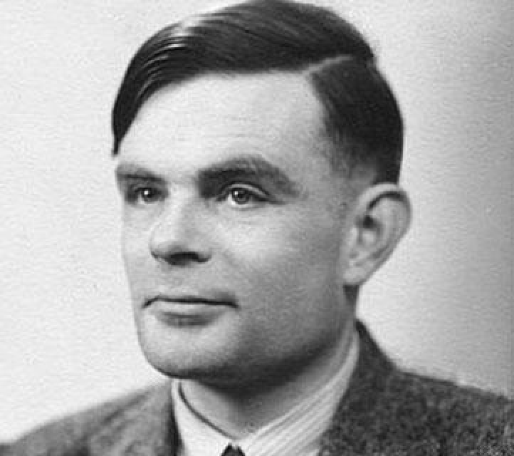
텍스트에 사전 훈련된 언어 분류기를 사용합니다: |
Classify["Language","the house is blue","la maison est bleue","la casa es azul","das Haus ist blau","房子是蓝色的","المنزل باللون الأزرق","будинок синій"]
사전 훈련된 모델은 다음과 같은 여러 다른 기능에 사용할 수 있습니다: |
ImageIdentify
,
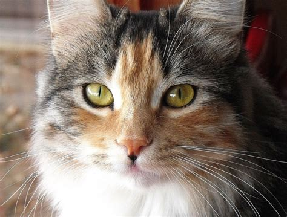
,
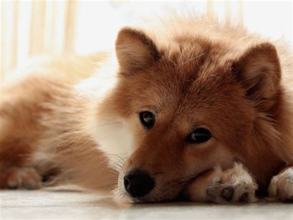
,SpecificityGoal->"Low"
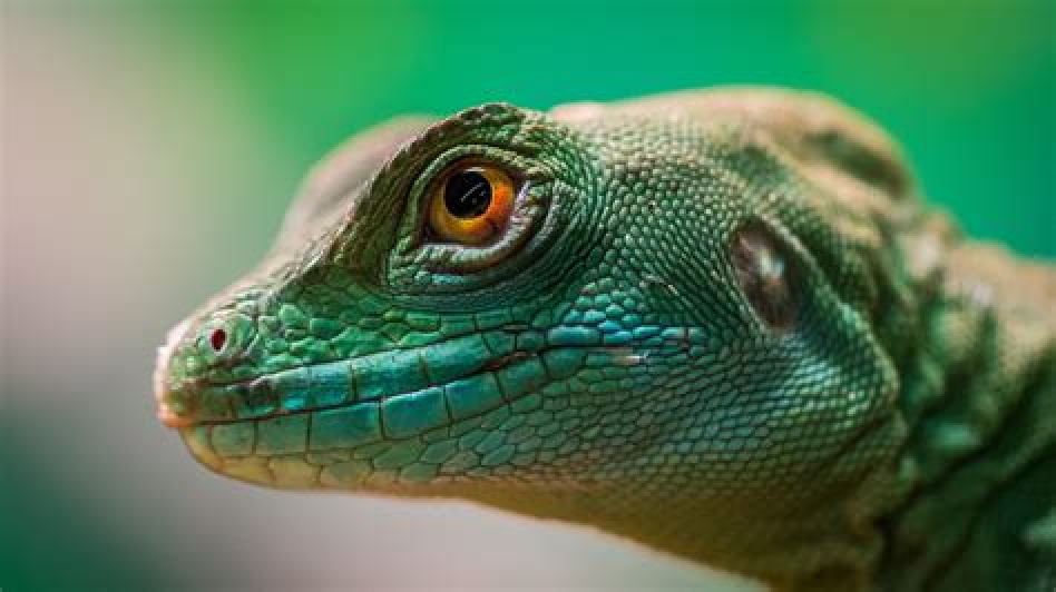
고수준 코드로 분류기를 직접 훈련합니다: |
topicClassifier=Classify"the cat is grey"->
,"my cat is fast"->

,"this dog is scary"->
,"the big dog"->

훈련된 모델을 사용합니다: |
topicClassifier[{"nice cat","what a dog"}]
클러스터 분석
클러스터 분석
데이터에서 클러스터를 찾습니다: |
ListPlotFindClusters
더욱 강력한 제어를 위해 방법 및 기타 옵션을 지정합니다: |
ListPlotFindClusters,Method->"DBSCAN"
그래프의 맥락에서 클러스터를 분석합니다: |
CommunityGraphPlot[ExampleData[{"NetworkGraph","JazzMusicians"}]]
이미지의 구성 요소를 분석합니다: |
ClusteringComponents
,7//Colorize
차원 축소
차원 축소
색상 함수는 데이터 구조가 더 낮은 차원 공간에 포함될 수 있음을 보여 줍니다: |
ListPointPlot3D,ColorFunction->Hue0.5-0.5
Total[]
&,ColorFunctionScaling->False,2
{#1,#2}
이 데이터 세트에 대한 차원 축소 함수를 만듭니다: |
dr=DimensionReduction,Method->"Isomap"
데이터에 차원 축소 함수를 적용합니다: |
ListPlotdr,ColorFunction(Hue[0.5#1]&)
이상 데이터 감지
이상 데이터 감지
클래식 데이터 세트에서 정보를 검색합니다: |
In[]:=
irisdata=ResourceData["Sample Data: Fisher's Irises"][All,{"PetalLength","SepalWidth"},QuantityMagnitude];
이상 감지 기능을 만듭니다: |
detector=AnomalyDetection[irisdata]
detector 함수를 사용하여 데이터 세트에서 이상을 찾습니다: |
anomalies=FindAnomalies[detector,irisdata]
데이터와 결정 경계를 시각화합니다: |
ShowContourPlotdetector[{x,y},"RarerProbability"],{x,-1,9},{y,1,5},,ListPlot{irisdata,anomalies},
누락된 데이터에 대한 값 대입
누락된 데이터에 대한 값 대입
데이터 세트에서 일부 정보를 제거하여 누락된 데이터를 시뮬레이션합니다: |
incompletedata=/.{x_/;4<x<5,y_}:>{x,Missing[]};ListPlot[incompletedata]
누락된 값을 예측하기 위한 분포를 학습합니다: |
{nonmissingdata,missingdata}=GatherBy[incompletedata,MemberQ[_Missing]];ld=LearnDistribution[nonmissingdata]
누락된 값을 합성하고 결과를 표시합니다: |
synthesized=SynthesizeMissingValues[ld,missingdata];ListPlot[{incompletedata,synthesized}]
신경망 훈련 및 연구
신경망 훈련 및 연구
분류를 위한 클래식 데이터 세트를 검색합니다: |
In[]:=
trainingdata=ResourceData["MNIST","TrainingData"];testdata=ResourceData["MNIST","TestData"];SeedRandom[1234];RandomSample[trainingdata,5]
Out[]=
9,

4,

0,

2,

5

데이터에 대한 모델을 학습합니다 (평가하는 데 시간이 오래 걸릴 수 있음): |
In[]:=
trainedNet=NetTrain[NetModel["LeNet"],trainingdata,MaxTrainingRounds->2]
Out[]=
NetChain


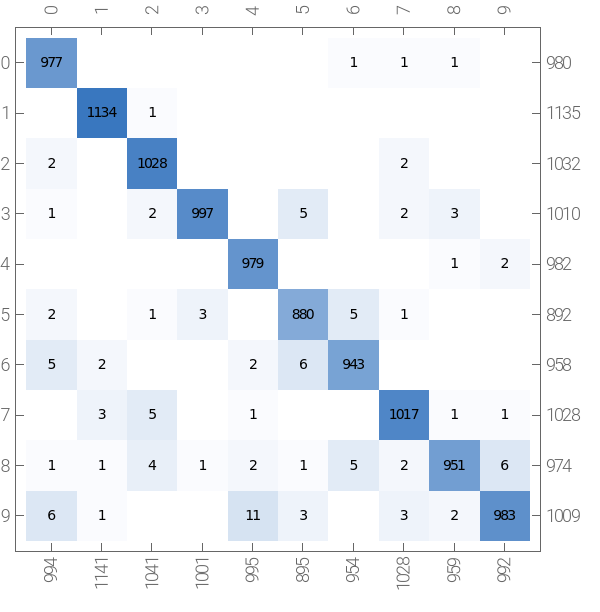
훈련된 네트워크의 성능을 살펴봅니다: |
NetMeasurements[trainedNet,testdata,{"Accuracy","ConfusionMatrixPlot"}]
Out[]=
0.9889,
actual class | |
| predicted class |
컴퓨터 비전
컴퓨터 비전
자연어 처리
자연어 처리
음성 분석
음성 분석