Wolfram 機械学習 | 試してみよう
Wolfram 機械学習 | 試してみよう
コードはどれも,コード内をクリックしてから,編集したり, を押して実行したりできます.
+
機械学習とニューラルネットワーク 従来の機械学習,統計解析,可視化,画像処理等と緊密に統合されている最新のAIを使って,生産グレードのインテリジェントなシステムが構築できます.
分類器を使い訓練する
分類器を使い訓練する
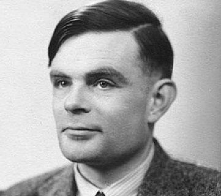
訓練済みの分類器を使って画像を識別する: |
Classify"NotablePerson",
テキストに訓練済みの言語分類器を使う: |
Classify["Language","the house is blue","la maison est bleue","la casa es azul","das Haus ist blau","房子是蓝色的","المنزل باللون الأزرق","будинок синій"]
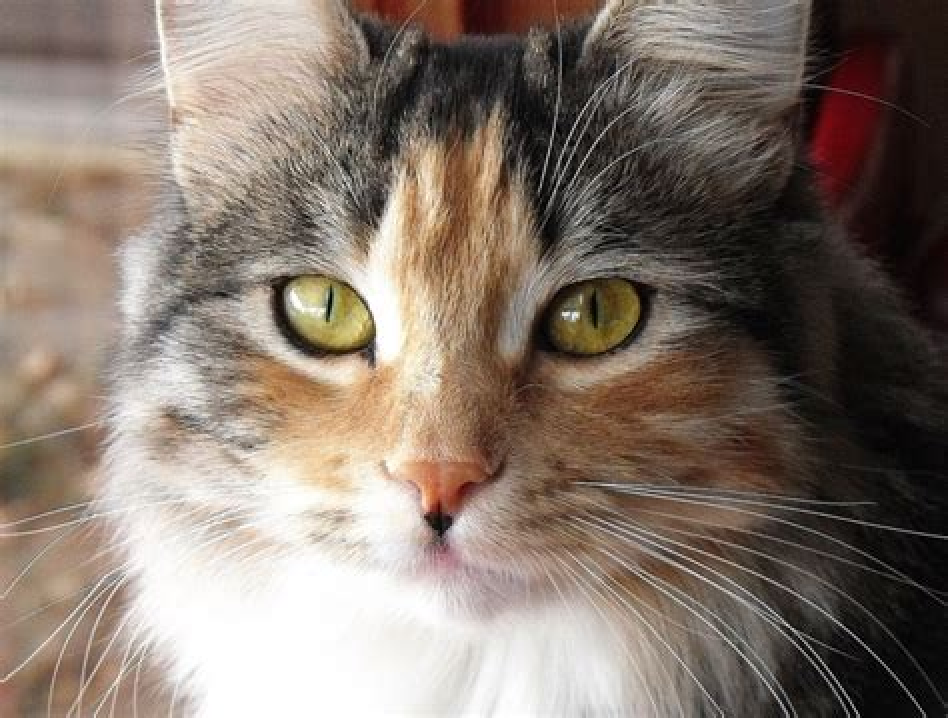
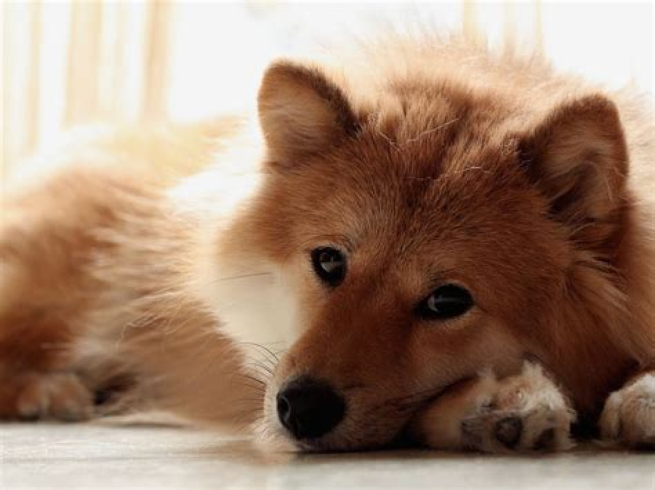
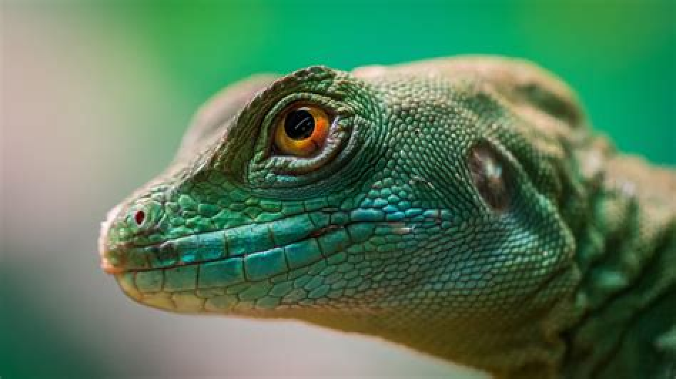
訓練済みモデルは他の多数の関数で使われる: |
ImageIdentify
,
,
,SpecificityGoal->"Low"
自作の分類器を高レベルのコードで訓練する: |
topicClassifier=Classify"the cat is grey"->
,"my cat is fast"->

,"this dog is scary"->
,"the big dog"->

訓練された自作モデルを使う: |
topicClassifier[{"nice cat","what a dog"}]
クラスタ分析
クラスタ分析
データのクラスタを見付ける: |
ListPlotFindClusters
よりよく制御するためにメソッドや他のオプションを指定する: |
ListPlotFindClusters,Method->"DBSCAN"
グラフにおけるクラスタを分析する: |
CommunityGraphPlot[ExampleData[{"NetworkGraph","JazzMusicians"}]]
画像の要素を分析する: |
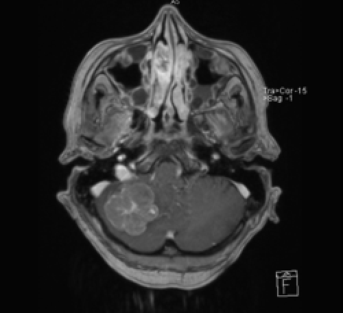
ClusteringComponents
,7//Colorize
次元削減
次元削減
色関数は,データの構造を低次元空間に埋め込むことができることを示している: |
ListPointPlot3D,ColorFunction->Hue0.5-0.5
Total[]
&,ColorFunctionScaling->False,2
{#1,#2}
このデータ集合についての次元削減関数を作成する: |
dr=DimensionReduction,Method->"Isomap"
データに次元削減関数を適用する: |
ListPlotdr,ColorFunction(Hue[0.5#1]&)
異常なデータを検出する
異常なデータを検出する
よく知られたデータ集合から情報を取得する: |
In[]:=
irisdata=ResourceData["Sample Data: Fisher's Irises"][All,{"PetalLength","SepalWidth"},QuantityMagnitude];
異常検出関数を作成する: |
detector=AnomalyDetection[irisdata]
検出関数を使って,データ集合内の異常値を見付ける: |
anomalies=FindAnomalies[detector,irisdata]
データと決定境界を可視化する: |
ShowContourPlotdetector[{x,y},"RarerProbability"],{x,-1,9},{y,1,5},,ListPlot{irisdata,anomalies},
欠損データの値を補完する
欠損データの値を補完する
データ集合から何らかの情報を削除して,欠損データを含むようにする: |
incompletedata=/.{x_/;4<x<5,y_}:>{x,Missing[]};ListPlot[incompletedata]
分布を訓練して欠損値を予測する: |
{nonmissingdata,missingdata}=GatherBy[incompletedata,MemberQ[_Missing]];ld=LearnDistribution[nonmissingdata]
欠損値を合成して結果をプロットする: |
synthesized=SynthesizeMissingValues[ld,missingdata];ListPlot[{incompletedata,synthesized}]
ニューラルネットワークを訓練して調べる
ニューラルネットワークを訓練して調べる
分類のためによく知られたデータ集合を取得する: |
In[]:=
trainingdata=ResourceData["MNIST","TrainingData"];testdata=ResourceData["MNIST","TestData"];SeedRandom[1234];RandomSample[trainingdata,5]
Out[]=
9,

4,

0,

2,

5

そのデータでモデルを訓練する(この評価には時間がかかる場合がある): |
In[]:=
trainedNet=NetTrain[NetModel["LeNet"],trainingdata,MaxTrainingRounds->2]
Out[]=
NetChain


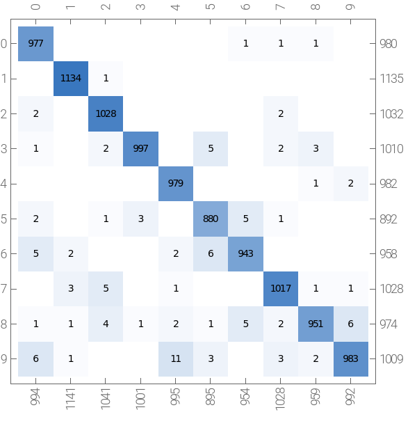
訓練されたネットワークの性能を見てみる: |
NetMeasurements[trainedNet,testdata,{"Accuracy","ConfusionMatrixPlot"}]
Out[]=
0.9889,
actual class | |
| predicted class |
コンピュータビジョン
コンピュータビジョン
自然言語処理
自然言語処理
音声解析
音声解析