Wolfram 知识库 | 应用示例
Wolfram 知识库 | 应用示例
在代码中点击并按下 ,即可编辑并运行任何代码。
+
即时访问真实世界的数据。与整个 Wolfram 语言无缝集成,使用数百个重要领域中不断增加的精心收集的数据进行计算并将其可视化。
使用地理数据进行计算
使用地理数据进行计算
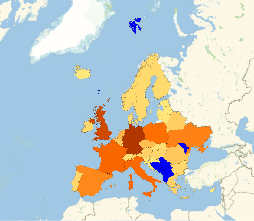
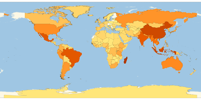
创建包含地理数据的地图(此计算可能需要较长时间): |
In[]:=
GeoRegionValuePlot->"GreenhouseGasEmissions",MissingStyle->Blue

Out[]=
获取每个国家的数据集合: |
In[]:=
rawdata=EntityValueEntityClass["Country","Countries"],,,,;

删除缺失数据并按大洲分组: |
In[]:=
cleandata=GroupBy[DeleteMissing[rawdata,1,1],Last,MapApply[Function[{pov,gdp,pop},{pov,QuantityMagnitude[gdp],pop}]]];
绘制清理后的数据: |
In[]:=
BubbleChartcleandata,
使用物理量进行计算
使用物理量进行计算
获取某类谱线的波长数据: |
In[]:=
wavelengths=EntityValue,;
在可见光谱范围内绘制这些谱线: |
In[]:=
GraphicsMap[{ColorData["VisibleSpectrum"][#],Line[{{#,0},{#,1}}]}&,QuantityMagnitude[wavelengths,"Nanometers"]],
获取物质的热力学数据: |
In[]:=
substances={"Water","Methanol","Octane"};temps=Quantity[Range[1,130],"DegreesCelsius"];densitydata=Table[{temps,ThermodynamicData[substance,"Density",{"Temperature"->temps}]}//Transpose,{substance,substances}];
可视化获取的数据: |
In[]:=
ListLinePlot[densitydata,AxesLabel->Automatic,PlotLegends->substances]
将图中密度骤降点与已知沸点进行比较: |
In[]:=
EntityValue[Interpreter["Chemical"][substances],"BoilingPoint","Association"]
使用生物与生态数据计算
使用生物与生态数据计算
在三维空间中绘制解剖结构的位置: |
In[]:=
AnatomyPlot3D,
比较解剖实体: |
In[]:=
organs=,,;properties={"Mass","CellCount"};ListPlot[EntityValue[organs,properties,"Association"],AxesLabel->properties]
定义生物序列并探索其结构特性: |
In[]:=
insulin=;MoleculePlot[Molecule[insulin]]
定义用于数据检索的实体类: |
In[]:=
endangeredMammal=EntityClass"TaxonomicSpecies",->,->;
直观了解各国濒危哺乳动物的数量: |
In[]:=
GeoRegionValuePlot[EntityValue[endangeredMammal,"ObservationCountries"]//Flatten//Tally]
Out[]=
分析金融数据
分析金融数据
获取金融数据并以标准格式呈现: |
In[]:=
TradingChart["GE",{"Volume","SimpleMovingAverage","BollingerBands"}]
从文本中解析金融实体: |
In[]:=
stocks=Interpreter["Financial"][{"GOOGL","MSFT","AAPL"}]
比较实体属性随时间的变化: |
In[]:=
property=;DateListPlotEntityValuestocks,Datedproperty,Interval,Yesterday,PlotLegendsCommonName[stocks]
使用社会文化数据计算
使用社会文化数据计算
可视化艺术家的流派偏好: |
In[]:=
genres=EntityValueEntityClass"Artwork","Artist"->,"ArtGenre"//Flatten;PieChart[Counts[genres],ChartLabels->Automatic]
从隐式定义的城堡类中获取建造起始日期: |
In[]:=
castleAndYear=EntityValueEntityClass"Castle",->,"ConstructionStartDate","NonMissingEntityAssociation";
分析时间趋势: |
In[]:=
DateHistogram[castleAndYear,{{900},{1300},"Decade"}]
整理特定活跃时期的数据: |