Wolfram 지식 기반 | 시도해 볼 것들
Wolfram 지식 기반 | 시도해 볼 것들
모든 코드는 클릭 한 다음 를 눌러 편집하거나 실행할 수 있습니다.
+
현실 세계 데이터에 즉시 접근 수백 가지 주요 도메인의 신중하게 엄선된 데이터 컬렉션은 Wolfram 언어 전체와 원활하게 통합되어 이를 사용하여 계산하고 시각화합니다.
지리 데이터로 계산하기
지리 데이터로 계산하기
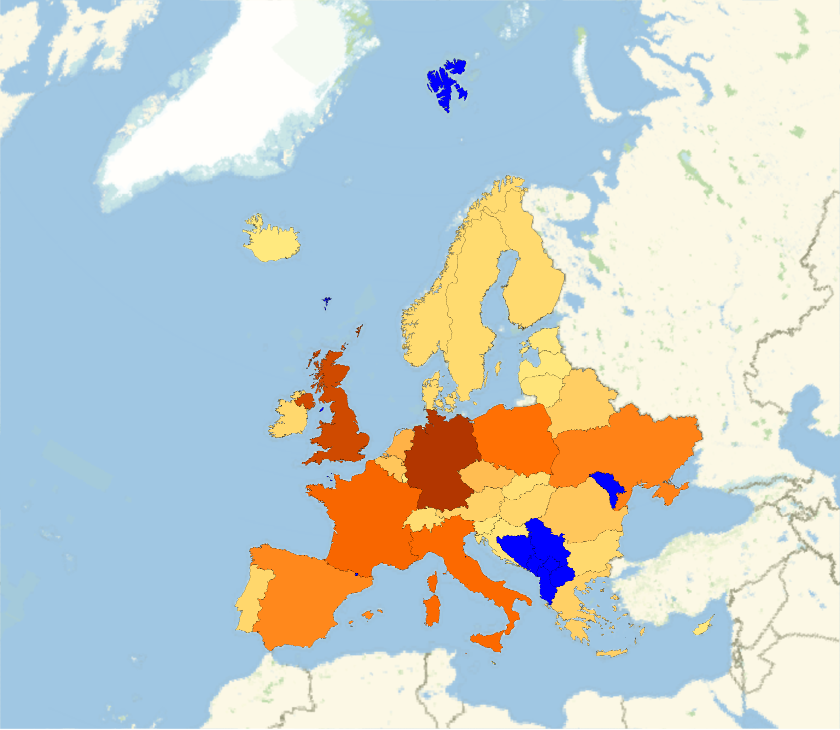
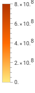
지리 데이터를 사용하여 지도를 만듭니다 (평가하는 데 시간이 오래 걸릴 수 있음): |
In[]:=
GeoRegionValuePlot->"GreenhouseGasEmissions",MissingStyle->Blue

Out[]=
각 국가에 대한 데이터 컬렉션을 검색합니다: |
In[]:=
rawdata=EntityValueEntityClass["Country","Countries"],,,,;

누락된 데이터를 삭제하고 대륙별로 그룹화합니다: |
In[]:=
cleandata=GroupBy[DeleteMissing[rawdata,1,1],Last,MapApply[Function[{pov,gdp,pop},{pov,QuantityMagnitude[gdp],pop}]]];
정리된 데이터를 플로팅합니다: |
In[]:=
BubbleChartcleandata,
물리량으로 계산하기
물리량으로 계산하기
스펙트럼 선 클래스에 대한 파장을 검색합니다: |
In[]:=
wavelengths=EntityValue,;
가시광선 스펙트럼에 다음 선을 표시합니다: |
In[]:=
GraphicsMap[{ColorData["VisibleSpectrum"][#],Line[{{#,0},{#,1}}]}&,QuantityMagnitude[wavelengths,"Nanometers"]],
물질에 대한 열역학 데이터를 검색합니다: |
In[]:=
substances={"Water","Methanol","Octane"};temps=Quantity[Range[1,130],"DegreesCelsius"];densitydata=Table[{temps,ThermodynamicData[substance,"Density",{"Temperature"->temps}]}//Transpose,{substance,substances}];
검색된 데이터를 시각화합니다: |
In[]:=
ListLinePlot[densitydata,AxesLabel->Automatic,PlotLegends->substances]
플롯에서 급격한 밀도 감소를 알려진 비등점과 비교합니다: |
In[]:=
EntityValue[Interpreter["Chemical"][substances],"BoilingPoint","Association"]
생물학 및 생태학 데이터로 계산하기
생물학 및 생태학 데이터로 계산하기
3D로 해부학적 구조의 위치를 표시합니다: |
In[]:=
AnatomyPlot3D,
해부학적 개체를 비교합니다: |
In[]:=
organs=,,;properties={"Mass","CellCount"};ListPlot[EntityValue[organs,properties,"Association"],AxesLabel->properties]
바이오시퀀스를 정의하고 구조적 특성을 살펴봅니다: |
In[]:=
insulin=;MoleculePlot[Molecule[insulin]]
데이터 검색을 위한 엔터티 클래스를 정의합니다: |
In[]:=
endangeredMammal=EntityClass"TaxonomicSpecies",->,->;
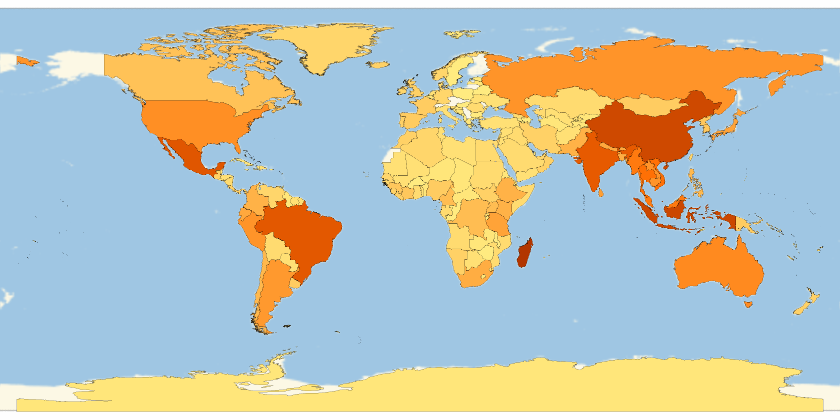
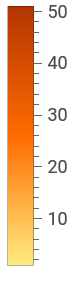
국가별로 멸종 위기에 처한 포유류의 수를 시각화합니다: |
In[]:=
GeoRegionValuePlot[EntityValue[endangeredMammal,"ObservationCountries"]//Flatten//Tally]
Out[]=
재무 데이터 분석
재무 데이터 분석
재무 데이터를 검색하여 표준 형식으로 표시합니다: |
In[]:=
TradingChart["GE",{"Volume","SimpleMovingAverage","BollingerBands"}]
텍스트에서 금융 기관을 해석합니다: |
In[]:=
stocks=Interpreter["Financial"][{"GOOGL","MSFT","AAPL"}]
시간에 따른 엔터티의 속성을 비교합니다: |
In[]:=
property=;DateListPlotEntityValuestocks,Datedproperty,Interval,Yesterday,PlotLegendsCommonName[stocks]
사회문화 데이터로 계산하기
사회문화 데이터로 계산하기
아티스트의 장르 선호도를 시각화합니다: |
In[]:=
genres=EntityValueEntityClass"Artwork","Artist"->,"ArtGenre"//Flatten;PieChart[Counts[genres],ChartLabels->Automatic]
암묵적으로 정의된 성 클래스에서 건설 시작 날짜를 검색합니다: |
In[]:=
castleAndYear=EntityValueEntityClass"Castle",->,"ConstructionStartDate","NonMissingEntityAssociation";
시간의 추세를 살펴봅니다: |
In[]:=
DateHistogram[castleAndYear,{{900},{1300},"Decade"}]
특히 활동적인 기간의 데이터를 구성합니다: |