
The latest versions of the Wolfram Language have built-in knowledge about singularities and branch cuts of mathematical functions. Here we show some examples of how this knowledge is used to solve univariate transcendental equations.
Suppose we would like to find all roots of a univariate function in a complex rectangle. We can start by finding root approximations using a numeric method. However, we would like to know for sure that each approximation represents an actual root and that we have found all the roots. This is where some knowledge of the function is required.
If we know that the function is holomorphic (complex differentiable) in the disk represented by an approximate number, we can use interval arithmetic (for elementary functions) or significance arithmetic (for non-elementary functions) and a criterion based on Rouché’s theorem to prove existence and the total multiplicity of roots in the disk.
To prove that we have found all the roots in a given complex rectangle, we compute the winding number of the function along the boundary of the rectangle (the total number of times that the value of the function travels around zero when its argument travels around the boundary of the rectangle) using interval arithmetic (for elementary functions) or numeric integration (for non-elementary functions). For this method to be valid, we need to know that the function is holomorphic in the rectangle or that the function is meromorphic (a ratio of holomorphic functions) in the rectangle, and we need to know the total multiplicity of poles of the function contained in the rectangle.
Holomorphic Function Example
Holomorphic Function Example
Using the built-in knowledge about mathematical functions, Solve can decide that is holomorphic in ( is given by cos(π/2)dt ). Since the function is not elementary, numeric integration is used to compute the winding number—hence the warning message:
FresnelC[z]-z-1
-2≤Re[z]≤2∧-2≤Im[z]≤2
FresnelC[z]
z
∫
0
2
t
sols=Solve[FresnelC[z]-z1&&-2≤Re[z]≤2&&-2≤Im[z]≤2,z]

Out[1]=
{{zRoot[{1-FresnelC[#1]+#1&,-1.47187658130381999332185573786}]},{zRoot[{1-FresnelC[#1]+#1&,-0.49779009060454277829015476190858119245805799298380655659705-1.22884790421709205702974277155375855473381605440648947973374}]},{zRoot[{1-FresnelC[#1]+#1&,-0.49779009060454277829015476190858119245805799298380655659705+1.22884790421709205702974277155375855473381605440648947973374}]},{zRoot[{1-FresnelC[#1]+#1&,0.99701104920390363530014302748685108318160770995138382725731-0.76819101638090424674595944289406300579269496443262030456307}]},{zRoot[{1-FresnelC[#1]+#1&,0.99701104920390363530014302748685108318160770995138382725731+0.76819101638090424674595944289406300579269496443262030456307}]}}
The roots are represented as Root objects , where is a pure function and is an approximate real or complex number such that exactly one root of lies within the numerical region defined by its precision. represents an exact number. In particular, we can compute its approximation to arbitrarily many digits:
Root[{f,}]
x
0
f
x
0
f[x]
Root[{f,}]
x
0
N[Root[{1-FresnelC[#1]+#1&,-1.47187658130381999332185573786}],100]
Out[2]=
-1.471876581303819993321855737858406345379922676272187672997702161972549246163460789585462914716272079
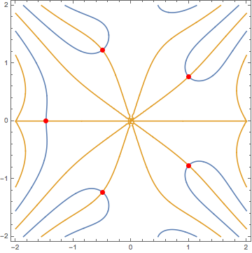
This illustrates the fact that the roots are intersection points of the zero sets of the real part and the imaginary part of the function:
In[3]:=
f=FresnelC[x+Iy]-x-Iy-1;
Show[{ContourPlot[{Re[f],Im[f]},{x,-2,2},{y,-2,2},Contours0,PlotPoints50],Graphics[{Red,PointSize[Large],Point[{Re[z],Im[z]}/.sols]}]}]
Out[4]=
Meromorphic Function Example
Meromorphic Function Example
Using the built-in knowledge about mathematical functions, Solve can decide that is meromorphic in and has two simple poles in the rectangle—at and . The function is elementary, so the winding number computation does not rely on approximate methods:
Tan[z]-Log[z+3]-
2
z
-2≤Re[z]≤2∧-2≤Im[z]≤2
-
π
2
π
2
sols=Solve[Tan[z]-Log[z+3]&&-2≤Re[z]≤2&&-2≤Im[z]≤2,z]
2
z
Out[5]=
{{zRoot[{Log[3+#1]+-Tan[#1]&,-1.84542184175728163291417602042}]},{zRoot[{Log[3+#1]+-Tan[#1]&,0.22199736877942795125916032643378985527085430280553352988223-1.09283854791258795469499773507416140338108857803289450573394}]},{zRoot[{Log[3+#1]+-Tan[#1]&,0.22199736877942795125916032643378985527085430280553352988223+1.09283854791258795469499773507416140338108857803289450573394}]},{zRoot[{Log[3+#1]+-Tan[#1]&,1.249979418341933269243814194368}]}}
2
#1
2
#1
2
#1
2
#1
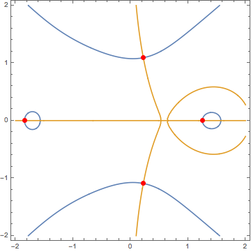
This illustrates the fact that the roots are intersection points of the zero sets of the real part and the imaginary part of the function. Note that and are not intersection points, since the function is not defined there:
-
π
2
π
2
In[6]:=
f=Tan[z]-Log[z+3]-z^2/.zx+Iy;
Show[{ContourPlot[{Re[f],Im[f]},{x,-2,2},{y,-2,2},Contours0,PlotPoints50],Graphics[{Red,PointSize[Large],Point[{Re[z],Im[z]}/.sols]}]}]
Out[7]=
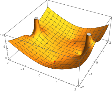
This shows the roots as minima of the absolute value:
Show[{Plot3D[Abs[f],{x,-2,2},{y,-2,2}],Graphics3D[{Red,PointSize[Large],Point[{Re[z],Im[z],0}/.sols]}]}]
Out[8]=
Root-Counting Examples
Root-Counting Examples
Here are some examples where the built-in knowledge about mathematical functions is used to count roots of holomorphic and meromorphic functions.
The roots are intersection points of the zero sets of the real part and the imaginary part of the function:
This shows the locations of roots and poles:
CountRoots uses FunctionPeriod to recognize periodicity. For periodic functions, it only needs to compute roots within one period and in the “remainder” rectangles: